Lecture 8 — A field approached through coupled oscillators

A chain of coupled harmonic oscillators is the simplest system in which the ground state of a local Hamiltonian is entangled across a spatial cut, and in which the number of degrees of freedom near the cut grows as the resolution improves. We develop the Gaussian formalism completely. For two oscillators the reduced state is obtained twice, from the wavefunction and from the covariance matrix, and it turns out to be exactly thermal for an oscillator that appears nowhere in the Hamiltonian. For many oscillators Williamson’s normal form reduces every regional state to independent thermal modes, and the modular Hamiltonian becomes an explicit quadratic form. A lattice experiment then separates what depends on the regulator from what does not: at fixed physical size the entropy of an interval grows as $\frac{1}{3}\log (1/a)$, while the mutual information of two separated intervals converges. The first fact is why Lecture 9 gives up regional density matrices; the second anticipates the split property. The modular spectrum of a half-chain, a ladder whose spacing closes as $a\to 0$, anticipates the boost of Lecture 10.

How to use this lecture

Classroom core, two meetings of two hours. The first meeting covers the motivation (§1, 10 minutes), two oscillators by the wavefunction (§2, 40 minutes) and by the covariance matrix (§3, 25 minutes), and the ground state of many oscillators with Williamson’s normal form (§§4.1–4.2, 35 minutes), leaving 10 minutes for Checkpoint 1. The second meeting covers the entropy and the modular Hamiltonian of a Gaussian state (§4.3, 15 minutes), the lattice field and its continuum limit (§§5.1–5.2, 25 minutes), the lattice experiment (§6, 40 minutes), and the scope of the result (§8, 10 minutes), with 30 minutes for Problems 3 and 4; Problems 1, 2, 5 and 6 complete the core assignment. These allocations are proposals and have not been tested in class.

Self-study. The zero mode and the infrared (§5.3), the half-chain and its modular ladder (§7), and Problems 7–12, including the entropy per endpoint from the corner-transfer-matrix spectrum.

Research extension. The lattice modular Hamiltonian near a cut, the mutual information as the gap closes, and the area law of a sphere, in Problems 13–15; Lecture 10 compares the lattice modular Hamiltonian with the continuum boost.

Prerequisites. Lecture 1 for restricted access, Lecture 3 for modular Hamiltonians and flows, Lecture 4 for entropy. Normal modes, the harmonic oscillator and Gaussian integrals.

What this lecture establishes. The reduced state of two oscillators and the entropy of a Gaussian regional state are exact calculations; Williamson’s normal form is proved for covariances without position–momentum correlations, which is the case of every ground state below. The lattice entropies of §6 are numerical results in an explicitly defined model, reproducible from the page. The two-dimensional conformal result $\frac{c}{3}\log (\ell /a)$ and the corner-transfer-matrix spectrum of the half-chain are stated with sources; the entropy per endpoint is then derived from that spectrum.

0. Reading

Primary.

• M. Srednicki, Entropy and Area (1993). The two-oscillator example of §2 is his.
• H. Casini, M. Huerta, Entanglement entropy in free quantum field theory (2009), the lattice formulas for Gaussian states and the two-dimensional results.
• I. Peschel, V. Eisler, Reduced density matrices and entanglement entropy in free lattice models (2009).

Secondary.

• L. Bombelli, R. K. Koul, J. Lee, R. D. Sorkin, Quantum source of entropy for black holes, Phys. Rev. D 34 (1986) 373.
• C. Holzhey, F. Larsen, F. Wilczek, Geometric and Renormalized Entropy in Conformal Field Theory (1994), and P. Calabrese, J. Cardy, Entanglement entropy and quantum field theory (2004).
• C. Weedbrook, S. Pirandola, R. García-Patrón, N. J. Cerf, T. C. Ralph, J. H. Shapiro, S. Lloyd, Gaussian Quantum Information (2011), for Williamson’s theorem and symplectic eigenvalues.
• K. Audenaert, J. Eisert, M. B. Plenio, R. F. Werner, Entanglement Properties of the Harmonic Chain (2002).

Optional research reading.

• I. Peschel, M.-C. Chung, Density Matrices for a Chain of Oscillators (1999), and I. Peschel, M. Kaulke, Ö. Legeza, Density-matrix spectra for integrable models (1998).
• H. Casini, M. Huerta, Entanglement and alpha entropies for a massive scalar field in two dimensions (2005).
• J. Eisert, M. Cramer, M. B. Plenio, Area laws for the entanglement entropy — a review (2008).
• V. Eisler, G. Di Giulio, E. Tonni, I. Peschel, Entanglement Hamiltonians for non-critical quantum chains (2020), and G. Di Giulio, E. Tonni, On entanglement hamiltonians of an interval in massless harmonic chains (2019).

1. Entropy behind a surface

In 1986 Bombelli, Koul, Lee and Sorkin asked whether the entropy of a black hole could be the entropy of quantum fields hidden behind its horizon. They took the vacuum of a free scalar field, traced out the field inside a sphere, and found an entropy proportional to the area of the sphere, with a coefficient set by the short-distance cutoff. Srednicki returned to the question in 1993, discretizing the field on radial shells, which turns it into a set of coupled harmonic oscillators, and evaluating the entropy numerically; his paper opens with the example of two oscillators that we work out in §2. The following year Holzhey, Larsen and Wilczek obtained the entropy of an interval in a two-dimensional conformal field theory, $\frac{c}{3}\log (\ell /a)$, and in 2004 Calabrese and Cardy rederived it with the replica trick and showed that in a massive theory it saturates at $\frac{c}{3}\log (\xi /a)$, with $\xi$ the correlation length.

A second line of work came from condensed matter, where the density-matrix renormalization group keeps the largest eigenvalues of reduced density matrices and the spectrum of those matrices became a practical question. Peschel and his collaborators showed that for free lattice models the reduced density matrix of half a chain is the exponential of a quadratic operator, and that its spectrum follows from Baxter’s corner transfer matrices of an associated two-dimensional model, a result we use in §7.

For this course the chain answers a question left by the finite codes of Lectures 1–7. Dividing three qutrits into shares is unambiguous, so why does dividing a quantum field into spatial regions require more care? The chain lets us perform the experiment with quantum mechanics alone: we fix a region of physical size, refine the lattice, and watch which quantities change. Three results of this lecture are used later. The entropy of a region diverges as the lattice spacing goes to zero, which motivates the algebraic description of Lecture 9. The mutual information of separated regions converges, which is the lattice shadow of the split property of the same lecture. And the modular Hamiltonian of a half-chain has a spectrum that becomes continuous in the limit, in the way the boost generator of Lecture 10 requires.

2. Two oscillators: the reduced wavefunction

Set $\hslash =1$ and take unit masses. Consider

$$H=\frac{1}{2}(p_1^2+p_2^2)+\frac{{\omega }_0^2}{2}(q_1^2+q_2^2)+\frac{\kappa }{2}(q_1-q_2{)}^2,[q_i,p_j]=i{\delta }_{ij},$$

with ${\omega }_0>0$ and $\kappa \ge 0$. The normal coordinates $q_{\pm }=(q_1\pm q_2)/\sqrt{2}$, and similarly $p_{\pm }$, preserve the commutators and decouple the Hamiltonian into two oscillators of frequencies

$${\omega }_{+}={\omega }_0,{\omega }_{-}=\sqrt{{\omega }_0^2+2\kappa }.$$

The ground state is the product of the two normal-mode ground states,

$${\psi }_0(q_1,q_2)={\left(\frac{{\omega }_{+}{\omega }_{-}}{{\pi }^2}\right)}^{1/4}\exp \left[-\frac{1}{2}\left({\omega }_{+}{q}_{+}^2+{\omega }_{-}{q}_{-}^2\right)\right],$$

and in the site variables the exponent reads $-\frac{1}{4}({\omega }_{+}+{\omega }_{-})(q_1^2+q_2^2)-\frac{1}{2}({\omega }_{+}-{\omega }_{-})q_1{q}_2$. The state factorizes between the normal modes and is entangled between the sites whenever $\kappa >0$. This is the distinction we met in Lecture 2 between the physical shares and the logical variables of a code.

An observer with access to site 1 alone sees the reduced density matrix. Its kernel is a Gaussian integral over the second site,

$${\rho }_1(q,q^{\prime })=\int d{q}_2{\psi }_0(q,q_2){\psi }_0(q^{\prime },q_2)=\sqrt{\frac{A-B}{\pi }}\exp \left[-\frac{A}{2}\left(q^2+q^{\prime 2}\right)+Bq{q}^{\prime }\right],$$

where

$$A=\frac{{\omega }_{+}^2+6{\omega }_{+}{\omega }_{-}+{\omega }_{-}^2}{4({\omega }_{+}+{\omega }_{-})},B=\frac{({\omega }_{+}-{\omega }_{-}{)}^2}{4({\omega }_{+}+{\omega }_{-})}.$$

To obtain them, complete the square in $q_2$: the integral of $\exp [-\alpha q_2^2-\beta q_2]$ with $\alpha =\frac{1}{2}({\omega }_{+}+{\omega }_{-})$ and $\beta =\frac{1}{2}({\omega }_{+}-{\omega }_{-})(q+q^{\prime })$ gives $\sqrt{\pi /\alpha }{e}^{{\beta }^2/4\alpha }$, and the term ${\beta }^2/4\alpha$ produces both the cross term and the reduction of the diagonal coefficient. Note that $A-B=2{\omega }_{+}{\omega }_{-}/({\omega }_{+}+{\omega }_{-})$, which fixes the normalization $\int dq{\rho }_1(q,q)=1$.

The kernel has the form of a thermal density matrix. For an oscillator $H_{\Omega }=\frac{1}{2}{p}^2+\frac{1}{2}{\Omega }^2{q}^2$, Mehler’s formula gives

$$⟨q|e^{-\beta H_{\Omega }}|q^{\prime }⟩=\sqrt{\frac{\Omega }{2\pi \sinh \beta \Omega }}\exp \left\{-\frac{\Omega }{2\sinh \beta \Omega }\left[(q^2+q^{\prime 2})\cosh \beta \Omega -2q{q}^{\prime }\right]\right\}.$$

Matching the two exponents requires $A=\Omega \coth \epsilon$ and $B=\Omega /\sinh \epsilon$, with $\epsilon =\beta \Omega$. Therefore ${\Omega }^2=A^2-B^2=(A-B)(A+B)$, and a short computation gives

$$\Omega =\sqrt{{\omega }_{+}{\omega }_{-}},\xi :=e^{-\epsilon }=\frac{B}{A+\Omega }={\left(\frac{\sqrt{{\omega }_{+}}-\sqrt{{\omega }_{-}}}{\sqrt{{\omega }_{+}}+\sqrt{{\omega }_{-}}}\right)}^2.$$

For the last step write $s=\sqrt{{\omega }_{+}}$ and $t=\sqrt{{\omega }_{-}}$; then $4(s^2+t^2)(A+\Omega )=s^4+6s^2{t}^2+t^4+4st(s^2+t^2)=(s+t{)}^4$, while $4(s^2+t^2)B=(s^2-t^2{)}^2$.

Thus the reduced state is exactly thermal,

$${\rho }_1=(1-\xi )\sum _{n=0}^{\infty }{\xi }^n|n_{\Omega }⟩⟨n_{\Omega }|,K_1=-\log {\rho }_1=\frac{\epsilon }{\Omega }{H}_{\Omega }-\frac{\epsilon }{2}-\log (1-\xi ),$$

where $|n_{\Omega }⟩$ are the number states of the oscillator of frequency $\Omega$. Its entropy is

$$S_1=-\log (1-\xi )-\frac{\xi }{1-\xi }\log \xi .$$

For ${\omega }_{-}/{\omega }_{+}=4$ we obtain $\xi =1/9$ and $S_1=\log \frac{9}{8}+\frac{1}{8}\log 9\approx 0.3924$.

Physical picture: thermal for a Hamiltonian nobody wrote down. The oscillator that diagonalizes ${\rho }_1$ has frequency $\sqrt{{\omega }_{+}{\omega }_{-}}$, the geometric mean of the normal modes. The Hamiltonian of site 1 by itself, $\frac{1}{2}{p}_1^2+\frac{1}{2}({\omega }_0^2+\kappa )q_1^2$, has frequency $\sqrt{{\omega }_0^2+\kappa }$, and the two agree only to first order in $\kappa$. The effective temperature $\Omega /\epsilon$ also depends on the coupling. What is exact is the statement about the modular Hamiltonian $K_1$: the restricted pure state is a Gibbs state of $K_1$ at unit temperature. Whether $K_1$ is proportional to a physical Hamiltonian is a separate question, and in Lecture 10 the answer for a relativistic wedge will be yes, with a boost in the role of $K_1$.

3. Two oscillators: the covariance matrix

The same result follows from second moments alone, and this second route is the one that generalizes. Since $⟨q_{\pm }^2⟩=1/(2{\omega }_{\pm })$ and $⟨p_{\pm }^2⟩={\omega }_{\pm }/2$, the covariance of site 1 is

$$X=⟨q_1^2⟩=\frac{1}{4}\left(\frac{1}{{\omega }_{+}}+\frac{1}{{\omega }_{-}}\right),P=⟨p_1^2⟩=\frac{1}{4}({\omega }_{+}+{\omega }_{-}),\frac{1}{2}⟨q_1{p}_1+p_1{q}_1⟩=0.$$

A Gaussian state is fixed by its first and second moments, so these three numbers determine ${\rho }_1$. The canonical rescaling $Q=(P/X{)}^{1/4}{q}_1$, $\Pi =(X/P{)}^{1/4}{p}_1$ preserves $[Q,\Pi ]=i$ and makes both variances equal to

$$\nu =\sqrt{XP}=\frac{{\omega }_{+}+{\omega }_{-}}{4\sqrt{{\omega }_{+}{\omega }_{-}}}.$$

Note that $(P/X{)}^{1/2}=\sqrt{{\omega }_{+}{\omega }_{-}}=\Omega$: the rescaling turns $q_1$ into the coordinate of the oscillator found in §2. A thermal oscillator with mean occupation $\bar{n}$ has $⟨Q^2⟩=⟨{\Pi }^2⟩=\bar{n}+\frac{1}{2}$. Therefore $\bar{n}=\nu -\frac{1}{2}$, and $\xi =\bar{n}/(\bar{n}+1)=(\nu -\frac{1}{2})/(\nu +\frac{1}{2})$. With $r={\omega }_{-}/{\omega }_{+}$ we have $\nu =\frac{1}{4}(\sqrt{r}+1/\sqrt{r})$, so that $\nu \mp \frac{1}{2}=(\sqrt{r}\mp 1{)}^2/(4\sqrt{r})$ and the ratio reproduces $\xi$ of §2. The entropy becomes

$$S_1=s(\nu ):=\left(\nu +\frac{1}{2}\right)\log \left(\nu +\frac{1}{2}\right)-\left(\nu -\frac{1}{2}\right)\log \left(\nu -\frac{1}{2}\right).$$

For $r=4$ we have $\nu =5/8$ and $\xi =1/9$, as before.

The number $\nu$ is invariant under local canonical rescalings, and it satisfies $\nu \ge \frac{1}{2}$ by the Robertson–Schrödinger uncertainty relation $XP-C^2\ge \frac{1}{4}$, with $C$ the symmetrized covariance of $q_1$ and $p_1$. For a single oscillator in a pure Gaussian state the bound is saturated. At $\kappa =0$ we obtain $\nu =\frac{1}{2}$, and for $\kappa >0$ the arithmetic–geometric mean inequality gives $\nu >\frac{1}{2}$.

Checkpoint 1. The total state is pure. Why is $\nu >\frac{1}{2}$ allowed for site 1?

Answer. Purity constrains the full covariance of both sites, whose two symplectic eigenvalues equal $\frac{1}{2}$. The covariance of site 1 omits the cross-correlations $⟨q_1{q}_2⟩$ and $⟨p_1{p}_2⟩$, and the restricted state is mixed.

4. Gaussian states of many oscillators

4.1 The ground-state covariance

For $N$ oscillators consider

$$H=\frac{1}{2}{p}^{T}p+\frac{1}{2}{q}^{T}Vq,$$

where $V$ is a real symmetric positive matrix. Write $V=O^T\mathrm{diag}({\omega }_k^2)O$ and rotate $q$ and $p$ by the same orthogonal matrix $O$, which preserves the commutators. Each normal mode contributes $1/(2{\omega }_k)$ to the position covariance and ${\omega }_k/2$ to the momentum covariance, and rotating back gives

$$X_{ij}=⟨q_i{q}_j⟩=\frac{1}{2}{\left(V^{-1/2}\right)}_{ij},P_{ij}=⟨p_i{p}_j⟩=\frac{1}{2}{\left(V^{1/2}\right)}_{ij},⟨q_i{p}_j+p_j{q}_i⟩=0.$$

The last relation holds because the ground-state wavefunction is real. Note that $XP=\frac{1}{4}$, the matrix form of the statement that the global state is pure.

For a set of sites $A$ the reduced state is Gaussian, with covariance given by the principal submatrices $X_A$ and $P_A$. Note that one must restrict after computing the square roots: restricting $V$ first would remove the couplings before finding the ground state, and it describes a different, isolated system (Problem 3).

4.2 Williamson’s normal form

The regional covariance can be brought to the diagonal form of §3 by a single canonical transformation.

Claim (Williamson’s normal form, block-diagonal case). Model proof. Let $X_A$ and $P_A$ be real symmetric positive matrices of size $n$, and write $X_A^{1/2}{P}_A{X}_A^{1/2}=O{D}^2{O}^T$ with $O$ orthogonal and $D=\mathrm{diag}({\nu }_1,\dots ,{\nu }_n)$ positive. The variables

$$Q=D^{1/2}{O}^T{X}_A^{-1/2}{q}_A,\Pi =D^{-1/2}{O}^T{X}_A^{1/2}{p}_A$$

are canonical, $[Q_i,{\Pi }_j]=i{\delta }_{ij}$, and in them

$$⟨Q{Q}^T⟩=⟨\Pi {\Pi }^T⟩=D,⟨Q_i{\Pi }_j+{\Pi }_j{Q}_i⟩=0.$$

Proof. The commutator matrix of $Q$ and $\Pi$ is $i{D}^{1/2}{O}^T{X}_A^{-1/2}{X}_A^{1/2}O{D}^{-1/2}=i1$, and $Q$, $\Pi$ are separately linear in $q_A$ and $p_A$, so they commute among themselves. The covariances are $D^{1/2}{O}^T{X}_A^{-1/2}{X}_A{X}_A^{-1/2}O{D}^{1/2}=D$ and $D^{-1/2}{O}^T(X_A^{1/2}{P}_A{X}_A^{1/2})O{D}^{-1/2}=D^{-1/2}{D}^2{D}^{-1/2}=D$. The mixed moments vanish because they vanish for $q_A$ and $p_A$. $\square$

Since $X_A^{1/2}{P}_A{X}_A^{1/2}$ is similar to $X_A{P}_A$, the symplectic eigenvalues ${\nu }_j$ are the positive square roots of the eigenvalues of $X_A{P}_A$, a matrix that need not be symmetric. Each ${\nu }_j\ge \frac{1}{2}$ by the uncertainty relation applied to the pair $(Q_j,{\Pi }_j)$. A computed value below $\frac{1}{2}$ signals an error in the covariance or insufficient precision, and it should be diagnosed before any logarithm is taken; clipping it would hide the error.

The general theorem, due to Williamson (1936), states that every positive covariance matrix, including one with position–momentum correlations, is brought to diagonal form by a symplectic transformation, and that its symplectic eigenvalues are the moduli of the eigenvalues of $i\sigma \gamma$, with $\gamma$ the covariance and $\sigma$ the symplectic form. We use only the block-diagonal case, which covers every ground state and every thermal state of a Hamiltonian of the form above. [Stated only — refs: Williamson 1936; Weedbrook et al. 2011.]

4.3 Entropy, modular Hamiltonian and Weyl operators

In the variables of the claim the Gaussian state is a product of thermal states, one for each pair $(Q_j,{\Pi }_j)$, since a Gaussian state is fixed by its moments and the product has the same moments. Therefore

$${\rho }_A=\underset{j=1}{\overset{n}{⨂}}(1-{\xi }_j){\xi }_j^{b_j^{†}{b}_j},S(A)=\sum _{j=1}^{n}s({\nu }_j),{\xi }_j=\frac{{\nu }_j-\frac{1}{2}}{{\nu }_j+\frac{1}{2}},$$

where $b_j=(Q_j+i{\Pi }_j)/\sqrt{2}$. This is a calculation with $n\times n$ matrices, although every oscillator has an infinite-dimensional Hilbert space.

The modular Hamiltonian is $K_A={\sum }_j{\epsilon }_j{b}_j^{†}{b}_j$ up to a constant, with ${\epsilon }_j=\log [({\nu }_j+\frac{1}{2})/({\nu }_j-\frac{1}{2})]$. Since $b_j^{†}{b}_j=\frac{1}{2}(Q_j^2+{\Pi }_j^2)-\frac{1}{2}$, substituting the claim gives a quadratic form in the original variables,

$$K_A=\frac{1}{2}{q}_A^{T}M{q}_A+\frac{1}{2}{p}_A^{T}N{p}_A+\text{constant},$$

where

$$M=X_A^{-1/2}O\mathrm{diag}({\nu }_j{\epsilon }_j)O^T{X}_A^{-1/2},N=X_A^{1/2}O\mathrm{diag}({\epsilon }_j/{\nu }_j)O^T{X}_A^{1/2}.$$

Two consequences are used later. The modular flow $e^{is{K}_A}(\cdot )e^{-is{K}_A}$ of a Gaussian state acts linearly on $q_A$ and $p_A$, by a symplectic transformation; in the continuum this becomes the statement that the modular flow of a free field acts on Weyl operators by a symplectic map of test functions, which Lecture 10 identifies with a boost. The second consequence is a numerical warning: modes deep inside the region have ${\nu }_j-\frac{1}{2}\simeq e^{-{\epsilon }_j}$ exponentially small, so the entropy is insensitive to them, while $M$ and $N$ require arithmetic with a precision beyond $e^{-{\epsilon }_{\max }}$. The lattice computations of modular Hamiltonians in the literature, and the one in Lecture 10, use high-precision arithmetic for this reason.

The state can also be described without density matrices, and this is the form that survives in the continuum. For real vectors $u,v$ define the Weyl operators

$$W(u,v)=\exp \left[i\left(u^{T}q+v^{T}p\right)\right],W(u,v)W(u^{\prime },v^{\prime })=e^{-i\sigma /2}W(u+u^{\prime },v+v^{\prime }),$$

where $\sigma =u^T{v}^{\prime }-v^T{u}^{\prime }$ is the symplectic form, fixed by $[u^{T}q+v^{T}p,u^{\prime T}q+v^{\prime T}p]=i\sigma$. In a centered Gaussian state without position–momentum correlations,

$$⟨W(u,v)⟩=\exp \left[-\frac{1}{2}\left(u^{T}Xu+v^{T}Pv\right)\right],$$

as follows for one thermal mode from $⟨e^{i(uQ+v\Pi )}⟩=e^{-\nu (u^2+v^2)/2}$ and for many modes from the linear transformation of the claim. The regional state is this characteristic function restricted to vectors $u,v$ supported in $A$. Lecture 9 defines the vacuum of the continuum field in exactly this way, with test functions in place of $u$ and $v$ and with no reference to a regional trace.

Finally, displacing the state leaves the entropy unchanged and shifts the expectation value of a quadratic $K_A$. For the state $W\rho W^{†}$ with $⟨q_A⟩=\delta q$ and $⟨p_A⟩=\delta p$, the relative entropy with respect to the undisplaced regional state is therefore

$$S({\rho }_{\delta ,A}\Vert {\rho }_A)=⟨K_A{⟩}_{\delta }-⟨K_A⟩=\frac{1}{2}\delta q^{T}M\delta q+\frac{1}{2}\delta p^{T}N\delta p.$$

For a single thermal mode this is $\epsilon |\alpha {|}^2$, with $\alpha$ the displacement of $b$ (Problem 9), and Lecture 10 computes the continuum limit of the formula for a half-line.

5. A chain and the limit that makes a field

5.1 The lattice field

Discretize a scalar field of mass $m$ on a periodic line of length $L=Na$, with

$$q_j=\sqrt{a}\varphi (ja),p_j=\sqrt{a}\pi (ja),$$

so that $[q_i,p_j]=i{\delta }_{ij}$ follows from $[\varphi (x),\pi (y)]=i\delta (x-y)$. The regulated Hamiltonian is

$$H_a=\frac{1}{2}\sum _{j=1}^N\left[p_j^2+m^2{q}_j^2+\frac{(q_{j+1}-q_j{)}^2}{a^2}\right],$$

and its normal-mode frequencies are

$${\omega }_k^2=m^2+\frac{4}{a^2}{\sin }^2\frac{\pi k}{N},k=0,\dots ,N-1.$$

For fixed physical momentum $2\pi k/L$ and $a\to 0$, this approaches $m^2+(2\pi k/L{)}^2$. Modes near the lattice cutoff, with momenta of order $1/a$, have no counterpart at fixed energy, but they are the ones that correlate neighboring sites across a cut.

A rescaling makes the lattice spacing disappear from every entropy. With ${\tilde{q}}_j=q_j/\sqrt{a}$ and ${\tilde{p}}_j=\sqrt{a}{p}_j$, which is canonical,

$$H_a=\frac{1}{a}\tilde{H},\tilde{H}=\frac{1}{2}\sum _j\left[{\tilde{p}}_j^2+(ma{)}^2{\tilde{q}}_j^2+({\tilde{q}}_{j+1}-{\tilde{q}}_j{)}^2\right].$$

The ground state is that of $\tilde{H}$, and local canonical rescalings do not change symplectic eigenvalues. Therefore the entropy of $n$ consecutive sites depends only on $ma$ and $n$, together with the global boundary conditions. On the infinite line the covariances of $\tilde{H}$ are

$${\tilde{X}}_{ij}={\int }_{-\pi }^{\pi }\frac{dk}{2\pi }\frac{e^{ik(i-j)}}{2\tilde{\omega }(k)},{\tilde{P}}_{ij}={\int }_{-\pi }^{\pi }\frac{dk}{2\pi }\frac{\tilde{\omega }(k)}{2}{e}^{ik(i-j)},\tilde{\omega }(k{)}^2=(ma{)}^2+4{\sin }^2\frac{k}{2}.$$

At fixed physical separation $|i-j|a=r$ and $a\to 0$, ${\tilde{X}}_{ij}=⟨\varphi (ia)\varphi (ja)⟩$ approaches the continuum two-point function $K_0(mr)/2\pi$. For $mr=1$ the lattice values are $0.066921$, $0.067003$ and $0.067008$ at $1/a=8$, $32$ and $128$, against $K_0(1)/2\pi =0.067008$.

5.2 What the limit holds fixed

A continuum limit fixes the physical mass, the lengths of the regions and their separations, and sends $a\to 0$. The number of sites in a region of length $\ell$ grows as $\ell /a$, and the dimensionless mass $ma$ goes to zero. But two other limits are easily confused with this one. Sending $N\to \infty$ at fixed $a$ is a thermodynamic limit of the lattice, which removes finite-size effects and keeps the cutoff. Keeping the number of sites of a region fixed while $a\to 0$ shrinks the region to a point. Only the first procedure asks what a region of a field theory contains.

5.3 The zero mode and the infrared

At $m=0$ the mode $k=0$ of the periodic chain has zero frequency, a free particle with no normalizable ground state, so the Gaussian formulas above do not apply. Dropping the mode silently changes the model; one may instead impose other boundary conditions, or treat a compact scalar with its zero mode handled separately.

On the infinite line the massless limit is also delicate, since the equal-point covariance grows logarithmically,

$${\tilde{X}}_{jj}=\frac{1}{2\pi }\log \frac{8}{ma}+O\left((ma{)}^2\log \frac{1}{ma}\right),$$

which is the infrared divergence of $⟨{\varphi }^2⟩$ for a massless scalar in two dimensions (Problem 12). Entropies of finite intervals stay finite for $m>0$, but at small $m\ell$ they acquire, besides the conformal term, a slowly varying contribution $\frac{1}{2}\log (-\log m\ell )$ found by Casini and Huerta. [Stated only — refs: Casini–Huerta 2005.] For this reason the lattice experiment below keeps $m>0$ and reads the universal coefficient from the dependence on $a$ at fixed $m\ell$.

6. Worked example: the entropy diverges, the mutual information converges

Take $m=1$, an interval $A$ of length $\ell =1$, and a second interval $B$ of the same length separated from $A$ by a gap $d=\frac{1}{2}$. For each lattice spacing we compute the covariances of §5.1, the symplectic eigenvalues of the principal submatrices for $A$, $B$ and $A\cup B$, and the entropies of §4.3. Every step is a finite matrix computation. In exact arithmetic every ${\nu }_j\ge \frac{1}{2}$; in double precision the deepest modes sit at $\frac{1}{2}$ to within rounding, about $10^{-15}$, and contribute nothing to the entropy. The results are

$1/a$	$S(A)$	increment	$I(A:B)$
8	0.68210	—	0.054376
16	0.91043	0.22833	0.054435
32	1.14067	0.23024	0.054430
64	1.37149	0.23082	0.054425
128	1.60247	0.23098	0.054424
256	1.83350	0.23103	0.054423
512	2.06455	0.23104	0.054423

where the increment is $S(A)$ minus its value at twice the spacing, and $I(A:B)=S(A)+S(B)-S(A\cup B)$ is the mutual information. The increments approach $\frac{1}{3}\log 2=0.231049$. That is,

$$S(A)=\frac{1}{3}\log \frac{\ell }{a}+\text{finite},$$

with the coefficient of the two-dimensional conformal result for $c=1$. The finite part depends on $m\ell$ and on the lattice, and it has no universal meaning. The mutual information converges to $0.054423$ within six digits.

A second experiment tests the massive saturation. For an interval much longer than the correlation length, $\ell =40/m$, the entropy at $ma=0.2,0.1,0.05,0.025,0.0125$ increases by $0.3245$, $0.3306$, $0.3325$ and $0.3331$ per halving of $ma$, in units of $\log 2$. The slope approaches $\frac{1}{3}$: the entropy of a long interval is $\frac{1}{3}\log (1/ma)$ plus a constant, the result of Calabrese and Cardy with $c=1$ and two endpoints, and the figure shows both behaviors.

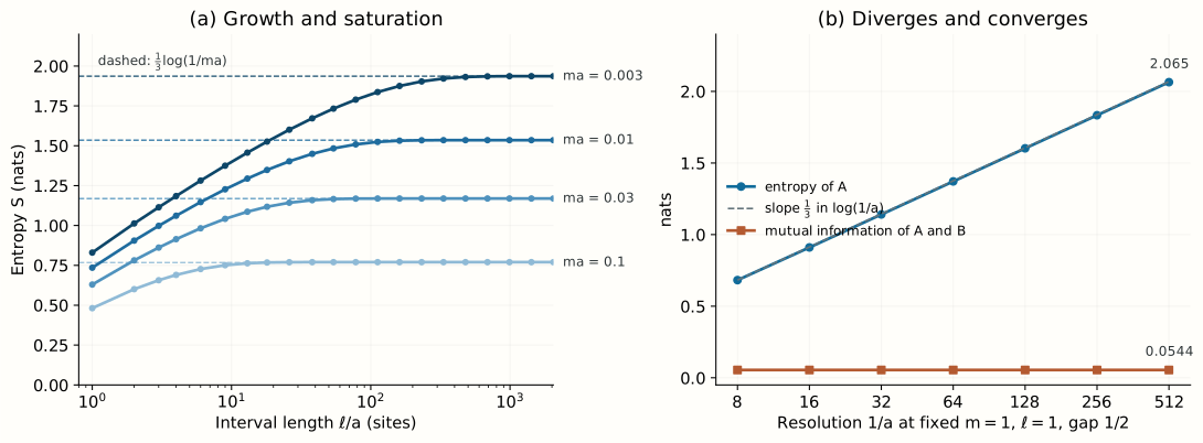
Checkpoint 2. Why does $I(A:B)$ converge while $S(A)$ diverges?

Answer. The divergent part of an entropy comes from correlations at distances of order $a$ across its endpoints. Separated intervals have $\partial (A\cup B)=\partial A\cup \partial B$, so the endpoint contributions cancel in $S(A)+S(B)-S(A\cup B)$. What remains measures correlations across the gap, at distances at least $d$, and these have a continuum limit.

Physical picture: entanglement at the shortest scale. The vacuum correlates neighboring points at every scale, and a sharp cut severs correlations at all wavelengths down to the cutoff. Each halving of $a$ adds a new layer of short-wavelength modes near each endpoint, and each layer contributes the same amount, $\frac{1}{6}\log 2$ per endpoint. A gap of fixed size removes those layers from the correlation between two regions. This is a statement about the lattice model and its numerics. In Lecture 9 the same contrast appears in algebraic form: for touching regions no type-I factor lies between $\mathcal{A}(O)$ and $\mathcal{A}(O^{\prime }{)}^{\prime }$, while a buffer supplies one under the hypotheses of the split property.

7. Self-study: the half-chain and its modular ladder

For the half-chain the regional spectrum is known in closed form: Peschel and Chung showed, using the corner transfer matrices of an associated two-dimensional Gaussian model, that the reduced density matrix of the sites $j\ge 1$ of the infinite chain $\tilde{H}$ is

$${\rho }_{\mathrm{half}}=\underset{j=0}{\overset{\infty }{⨂}}\left(1-e^{-{\epsilon }_j}\right)e^{-{\epsilon }_j{n}_j},{\epsilon }_j=(2j+1)\epsilon ,\epsilon =\pi \frac{K(k^{\prime })}{K(k)},$$

where $n_j$ are number operators of independent modes, $K$ is the complete elliptic integral of the first kind, and the modulus is fixed by $k+1/k=2+(ma{)}^2$, with $k^{\prime }=\sqrt{1-k^2}$. [Stated only — refs: Peschel–Chung 1999; Peschel–Eisler 2009.] The numerics of §6 confirm it. An interval of $1500$ sites at $ma=0.02$ is thirty correlation lengths long, so its two endpoints act as independent half-chains, and its lowest modular energies come in degenerate pairs $1.64727$, $4.94181$, $8.23635$; the formula gives $\epsilon =1.64727$ and the ratios $1:3:5$.

The entropy of the half-chain follows from this spectrum. Write $q=e^{-\epsilon }$ and

$$F(\epsilon )=-\sum _{j=0}^{\infty }\log \left(1-q^{2j+1}\right),S_{\mathrm{half}}=\sum _{j=0}^{\infty }{s}_j=\left(1-\epsilon \frac{d}{d\epsilon }\right)F(\epsilon ),$$

where $s_j={\epsilon }_j/(e^{{\epsilon }_j}-1)-\log (1-e^{-{\epsilon }_j})$ is the entropy of one thermal mode. The product is a ratio of Dedekind functions. With $\eta (\tau )=e^{i\pi \tau /12}{\prod }_{n\ge 1}(1-e^{2\pi in\tau })$ and $\tau =i\epsilon /2\pi$,

$$\prod _{j\ge 0}\left(1-q^{2j+1}\right)=q^{1/24}\frac{\eta (\tau )}{\eta (2\tau )}.$$

The modular transformation $\eta (-1/\tau )=\sqrt{-i\tau }\eta (\tau )$ converts the small-$\epsilon$ behavior into a rapidly convergent product, and one obtains (Problem 11)

$$F(\epsilon )=\frac{{\pi }^2}{12\epsilon }-\frac{1}{2}\log 2+\frac{\epsilon }{24}+O\left(e^{-2{\pi }^2/\epsilon }\right),S_{\mathrm{half}}=\frac{{\pi }^2}{6\epsilon }-\frac{1}{2}\log 2+O\left({\epsilon }^{-1}{e}^{-2{\pi }^2/\epsilon }\right).$$

For small $ma$ the modulus satisfies $k^{\prime 2}=2ma+O((ma{)}^2)$, so that $K(k^{\prime })\to \pi /2$ and $K(k)\simeq \log (4/k^{\prime })$. Thus

$$\epsilon \simeq \frac{{\pi }^2}{\log (8/ma)},S_{\mathrm{half}}\simeq \frac{1}{6}\log \frac{8}{ma}-\frac{1}{2}\log 2=\frac{1}{6}\log \frac{1}{ma},$$

since $\frac{1}{6}\log 8=\frac{1}{2}\log 2$. The values of $S_{\mathrm{half}}$ at $ma=0.1$, $0.02$ and $0.005$ are $0.38508$, $0.65208$ and $0.88306$, against $\frac{1}{6}\log (1/ma)=0.38376$, $0.65200$ and $0.88305$. The corrections are of order $(ma{)}^2\log (1/ma)$: the terms exponentially small in $1/\epsilon$ are of this size, since $e^{-2{\pi }^2/\epsilon }\simeq (ma/8{)}^2$, and ${\pi }^2/6\epsilon$ itself differs from $\frac{1}{6}\log (8/ma)$ by $(ma{)}^2/96$. Each endpoint therefore contributes $\frac{c}{6}\log (\xi /a)$ with $c=1$ and $\xi =1/m$, and an interval longer than $\xi$ has two of them, which is the saturation of §6.

But the spectrum carries more information than its entropy. The modular energies form a ladder of spacing $2\epsilon =2{\pi }^2/\log (8/ma)$, which closes as $a\to 0$, and the number of levels below a fixed modular energy grows as $\log (1/ma)$. The divergence of the entropy is the growth of this density of levels, and in the continuum the ladder becomes a continuous spectrum.

Physical picture: a lattice boost. Baxter’s corner transfer matrix transports a two-dimensional lattice model around a corner, and Thacker observed in 1986 that its generator is a lattice version of the Lorentz boost. The reduced density matrix of the half-chain is a product of corner transfer matrices that together turn the Euclidean plane by a full angle around the cut. Lecture 10 meets the same full turn as the origin of the factor $2\pi$ in the Bisognano–Wichmann relation $\Delta =e^{-2\pi K}$, where $K$ is the boost generator. This is a heuristic link. The lattice statements are those of Peschel and collaborators, and the continuum statement is the theorem of Lecture 10.

8. What the chain does and does not decide

At every finite lattice spacing, a set of sites carries a type-I algebra, a trace and a density matrix. Refining the lattice at fixed physical size makes its entropy grow without bound. The growth alone does not determine what algebra describes the region in the limit: the type of a limiting algebra depends on the observables retained, the state, and the representation in which the limit is taken, and Lecture 9 gives infinite-product examples with divergent entropy and different types.

What the calculation does establish is why the continuum question cannot be answered by keeping a fixed number of oscillators. At fixed physical length the number of modes near each endpoint grows as the spacing shrinks, and each new layer is entangled across the cut. The convergence of the mutual information and the closing of the modular ladder are lattice evidence for two continuum statements, the split property of Lecture 9 and the geometric modular flow of Lecture 10. They are evidence only; the continuum statements are theorems with their own hypotheses.

9. What to take away

• Exact calculation: the reduced state of one of two coupled oscillators is thermal for an oscillator of frequency $\sqrt{{\omega }_{+}{\omega }_{-}}$, with $e^{-\epsilon }={\left(\frac{\sqrt{{\omega }_{+}}-\sqrt{{\omega }_{-}}}{\sqrt{{\omega }_{+}}+\sqrt{{\omega }_{-}}}\right)}^2$; the wavefunction and the covariance give the same state.
• Model proof: a Gaussian state without position–momentum correlations is a product of thermal modes, with symplectic eigenvalues ${\nu }_j$ the square roots of the eigenvalues of $X_A{P}_A$; the entropy is ${\sum }_{j}s({\nu }_j)$, and the modular Hamiltonian is a quadratic form whose flow is symplectic.
• Numerical, in a defined model: at fixed physical sizes the increments of the interval entropy per halving of $a$ approach $\frac{1}{3}\log 2$, while the mutual information of separated intervals converges to six digits.
• Stated only, with an exact consequence: the half-chain has modular energies $(2j+1)\epsilon$ with $\epsilon \simeq {\pi }^2/\log (8/ma)$, and its entropy is $\frac{1}{6}\log (1/ma)+O((ma{)}^2\log (1/ma))$.
• Heuristic: divergent entropy does not classify the limiting algebra; convergent mutual information and a closing modular ladder anticipate the split property and the boost.

10. Looking ahead

Lecture 9 replaces the matrices $X_A$ and $P_A$ by the algebra generated by Weyl operators of test functions supported in a region, and the characteristic function of §4.3 by the vacuum state on that algebra; the divergence of §6 becomes the absence of a regional trace, and the convergence becomes the split property. Lecture 10 states the continuum result for the half-line, that the modular Hamiltonian of a Rindler wedge is $2\pi$ times the boost generator, and tests numerically that the lattice relative entropy of §4.3 approaches the boost energy of a classical wave. Lecture 23 reuses the effective thermal spectrum of §2, with a physical Hamiltonian in the role of $K_1$.

11. Problem set

Classroom core

1. The uncoupled limit. Show that $\nu =\frac{1}{2}$ if and only if ${\omega }_{+}={\omega }_{-}$, that is, $\kappa =0$.

2. Purity without a wavefunction integral. Compute $\mathrm{Tr}{\rho }_1^2$ from the spectrum of ${\rho }_1$ and express it in terms of $\nu$.

3. A principal submatrix does not commute with a function. For two oscillators compare $X_{11}$ with $1/\left(2\sqrt{V_{11}}\right)$ and explain which system each describes.

4. The Mehler match. Show that $A=\Omega \coth \epsilon$ and $B=\Omega /\sinh \epsilon$ imply $\Omega =\sqrt{A^2-B^2}$ and $e^{-\epsilon }=B/(A+\Omega )$, and verify $\Omega =\sqrt{{\omega }_{+}{\omega }_{-}}$ from the expressions for $A$ and $B$.

5. A numerical example. For ${\omega }_{-}/{\omega }_{+}=4$, compute $\nu$, $\xi$, $S_1$ and the effective temperature $\Omega /\epsilon$ in units of ${\omega }_{+}$.

6. Only $ma$ matters. Show that the symplectic eigenvalues of $n$ consecutive sites of $H_a$ depend on $a$ and $m$ only through $ma$. What does this imply for the entropy of an interval of fixed physical length as $a\to 0$?

Self-study consolidation

7. Weak coupling. Let $u=\kappa /{\omega }_0^2\ll 1$. Find the leading behavior of $\nu -\frac{1}{2}$ and of $S_1$, and explain why the entropy has no regular power series in $u$.

8. Williamson in two lines. For $X_A=\mathrm{diag}(x_1,x_2)$ and a nondiagonal $P_A$, construct the transformation of §4.2 explicitly and verify that it diagonalizes both covariances.

9. Relative entropy of a displacement. Show that $S({\rho }_{\delta ,A}\Vert {\rho }_A)=\frac{1}{2}\delta q^{T}M\delta q+\frac{1}{2}\delta p^{T}N\delta p$, and that for one thermal mode displaced by $\alpha$ it equals $\epsilon |\alpha {|}^2$.

10. Mutual information at large separation. Explain why $I(A:B)\ge 0$, and estimate how it decays when the gap $d$ is much larger than $1/m$. Hint: the mutual information of Gaussian states is quadratic in weak cross-correlations.

11. The modular transformation. Derive $F(\epsilon )=\frac{{\pi }^2}{12\epsilon }-\frac{1}{2}\log 2+\frac{\epsilon }{24}+O(e^{-2{\pi }^2/\epsilon })$ from the product formula of §7, and from it $S_{\mathrm{half}}=\frac{{\pi }^2}{6\epsilon }-\frac{1}{2}\log 2$ up to exponentially small terms.

12. The infrared. Show that ${\tilde{X}}_{jj}=\frac{1}{2\pi }\log \frac{8}{ma}$ up to corrections of order $(ma{)}^2\log (1/ma)$, and explain why the periodic massless chain has no normalizable Gaussian ground state.

Research extension

13. The modular Hamiltonian near a cut. Compute the kernels $M$ and $N$ of §4.3 for a long interval of the massive chain, with high-precision arithmetic, and compare them near one endpoint with the discretized boost generator $2\pi {\sum }_j{x}_j{h}_j$, where $h_j$ is the energy density at site $j$ and $x_j$ its distance from the cut. Known: Eisler, Di Giulio, Tonni and Peschel find dominant on-site and nearest-neighbor terms with triangular profiles, and small longer-range couplings that matter near criticality; Di Giulio and Tonni obtain the conformal result in the massless continuum limit. Completion: the profiles of the diagonal terms of $N$ and of the nearest-neighbor terms of $M$ for two masses, with the size of the longer-range terms.

14. When the gap closes. Compute $I(A:B)$ for two intervals of length $\ell$ as the gap $d$ decreases at fixed $a$, and as $a\to 0$ at fixed $d$. Known: for adjacent intervals the mutual information diverges as $a\to 0$, and Lecture 9 relates this to the absence of a type-I factor between touching regions; Hollands and Sanders bound entanglement measures in terms of the size of the buffer. Completion: the behavior of $I$ as a function of $d/\ell$ at small $d$, and the demonstration that the limits $a\to 0$ and $d\to 0$ do not commute.

15. The area law. Discretize a free massless scalar in $3+1$ dimensions on radial shells, as Srednicki did, and compute the entropy of a ball of radius $R$. Known: Srednicki finds an entropy proportional to $R^2/a^2$, with a coefficient of about $0.3$. Completion: the coefficient to a few percent, and the demonstration that the dependence on $R$ is quadratic over a decade.

12. Answer checkpoints

1. With $r={\omega }_{-}/{\omega }_{+}$, $\nu =\frac{1}{4}(\sqrt{r}+1/\sqrt{r})\ge \frac{1}{2}$ with equality only at $r=1$, which requires $\kappa =0$.

2. The geometric series gives $(1-\xi {)}^2/(1-{\xi }^2)=(1-\xi )/(1+\xi )=1/(2\nu )$, which is less than one for $\kappa >0$.

3. $X_{11}=\frac{1}{4}({\omega }_{+}^{-1}+{\omega }_{-}^{-1})$, while $1/(2\sqrt{V_{11}})=1/(2\sqrt{{\omega }_0^2+\kappa })$. They agree at $\kappa =0$ and differ at second order in $\kappa$. The second is the ground-state variance of site 1 with site 2 clamped, an isolated oscillator, and it has no entropy.

4. $A^2-B^2={\Omega }^2({\coth }^2\epsilon -{\sinh }^{-2}\epsilon )={\Omega }^2$, and $B/(A+\Omega )=1/(\cosh \epsilon +\sinh \epsilon )=e^{-\epsilon }$. With $A-B=2{\omega }_{+}{\omega }_{-}/({\omega }_{+}+{\omega }_{-})$ and $A+B=\frac{1}{2}({\omega }_{+}+{\omega }_{-})$, the product is ${\omega }_{+}{\omega }_{-}$.

5. $\nu =5/8$, $\xi =1/9$, $S_1=\log \frac{9}{8}+\frac{1}{8}\log 9\approx 0.3924$, $\Omega =2{\omega }_{+}$, $\epsilon =\log 9$, and $\Omega /\epsilon =2{\omega }_{+}/\log 9\approx 0.910{\omega }_{+}$.

6. The canonical rescaling ${\tilde{q}}_j=q_j/\sqrt{a}$, ${\tilde{p}}_j=\sqrt{a}{p}_j$ gives $H_a=\tilde{H}/a$, where $\tilde{H}$ contains only $ma$. The ground state does not depend on the overall factor $1/a$, and symplectic eigenvalues are invariant under local rescalings. An interval of length $\ell$ contains $\ell /a$ sites with $ma\to 0$, so its entropy is a function $S(\ell /a,ma)$, and the limit probes both arguments at once.

7. $r=\sqrt{1+2u}$ gives $\nu -\frac{1}{2}=\frac{u^2}{16}+O(u^3)$. With $n=\nu -\frac{1}{2}$, $s(\nu )=n(1-\log n)+O(n^2)$, so $S_1\simeq \frac{u^2}{16}\left(1-\log \frac{u^2}{16}\right)$. The logarithm reflects the nonanalyticity of $-x\log x$ at a pure state.

8. $X_A^{\pm 1/2}=\mathrm{diag}(x_1^{\pm 1/2},x_2^{\pm 1/2})$. Diagonalize the symmetric matrix $X_A^{1/2}{P}_A{X}_A^{1/2}=O{D}^2{O}^T$ and form $Q$ and $\Pi$; the two covariance computations of the proof in §4.2 apply entry by entry.

9. $S(W\rho W^{†})=S(\rho )$ because $W$ is unitary, so the relative entropy equals the change of $⟨K_A⟩$. A quadratic $K_A$ shifts by $\frac{1}{2}{\delta }^T(M\oplus N)\delta$, because the linear terms vanish in the centered state. For one mode $K=\epsilon b^{†}b$, and the displaced expectation value is $\epsilon (\bar{n}+|\alpha {|}^2)$.

10. $I(A:B)$ is the relative entropy between ${\rho }_{AB}$ and ${\rho }_A\otimes {\rho }_B$, and therefore nonnegative. The cross-correlations decay as $K_0(md)\sim e^{-md}$, and a second-order expansion in them gives $I\sim e^{-2md}$ times a power of $d$. For two intervals of length $1/m$, with $m=1$ as in §6 and $1/a=64$, the lattice gives $I=0.0133$, $0.00116$ and $0.000119$ at $md=1$, $2$ and $3$.

11. $\tau \mapsto -1/\tau$ sends $\tau =i\epsilon /2\pi$ to $2\pi i/\epsilon$, so that $\eta (\tau )=\sqrt{2\pi /\epsilon }{e}^{-{\pi }^2/6\epsilon }\left[1+O(e^{-4{\pi }^2/\epsilon })\right]$ and $\eta (2\tau )=\sqrt{\pi /\epsilon }{e}^{-{\pi }^2/12\epsilon }\left[1+O(e^{-2{\pi }^2/\epsilon })\right]$. The ratio is $\sqrt{2}{e}^{-{\pi }^2/12\epsilon }$, and $F=-\log \left(q^{1/24}\eta (\tau )/\eta (2\tau )\right)$ gives the stated series. Applying $1-\epsilon d/d\epsilon$ cancels the term linear in $\epsilon$ and doubles ${\pi }^2/12\epsilon$.

12. ${\tilde{X}}_{jj}=\frac{1}{2\pi }{\int }_0^{\pi }dk/\sqrt{(ma{)}^2+4{\sin }^2(k/2)}$ is a complete elliptic integral with modulus close to one; its logarithmic behavior gives $\frac{1}{2\pi }\log (8/ma)$. At $ma=10^{-3}$ the integral is $1.430357$ and the formula gives $1.430357$. On the periodic massless chain the mode $k=0$ has $V$-eigenvalue zero, so $X=\frac{1}{2}{V}^{-1/2}$ does not exist; that mode is a free particle, with continuous spectrum and no normalizable ground state.