Lecture 9 — Continuum algebras and separated regions

When the lattice of Lecture 8 is refined, the entropy of a region diverges while the mutual information of separated regions stays finite. This lecture explains both facts through the algebra of observables of a region. We build the local algebras of a free field from Weyl operators and define the vacuum by its characteristic function, with no regional trace. The Reeh–Schlieder theorem makes the vacuum cyclic for every region; we sketch why, prove that the vacuum is then separating, and show that the cyclicity cannot be used to signal. Infinite products of entangled pairs show that a divergent entropy does not decide the type of an algebra, and their modular spectra, which we compute, tell the types apart. Araki’s relative entropy survives the loss of the trace, and for a unitary excitation it equals a change of modular energy, the formula that Lecture 10 turns into the boost energy of a wave. A buffer between two regions restores a type-I factor, and with it product states and finite correlation measures.

How to use this lecture

Classroom core, two meetings of two hours. The first meeting covers the question and its history (§1, 10 minutes), the local algebras and the vacuum of a free field (§2, 35 minutes), the Haag–Kastler framework (§3, 15 minutes), and the cyclic and separating vacuum with the no-signaling argument (§§4.1, 4.3 and 4.4, 45 minutes), leaving 15 minutes for Checkpoint 1 and Problem 1. The second meeting covers the absence of a regional trace (§5.1, 10 minutes), infinite products and their modular spectra (§5.2, 35 minutes), relative entropy and unitary excitations (§§6.1–6.2, 35 minutes), and the split property (§7, 25 minutes), with 15 minutes for Checkpoint 2; Problems 2–6 complete the core assignment. These allocations are proposals and have not been tested in class.

Self-study. The analytic sketch of the Reeh–Schlieder theorem (§4.2), the Connes invariant and why one modular spectrum does not classify (§5.3), the properties of relative entropy (§6.3), and Problems 7–12.

Research extension. Correlation measures across a corridor, detector tests of a buffer, and the scaling route to type III${}_1$, in Problems 13–15.

Prerequisites. Lecture 1 for restricted access, Lecture 3 for the modular operator, $\hat{K}=-\log \Delta$ and the upper-strip convention, Lecture 5 for algebras with a center, Lecture 8 for Gaussian states and lattice Weyl operators. Hilbert-space completion and bounded operators.

What this lecture establishes. That the vacuum is separating given cyclicity, that local instruments cannot signal, the finite relative modular operator, the norm cost of cyclicity in a finite model, and the formula for the relative entropy of a unitary excitation are proved. The modular spectra of the infinite-product models are exact calculations; the classification of the factors they generate is stated with references. The Reeh–Schlieder theorem is sketched, with its analytic step named. The type III${}_1$ property of local algebras and the split property of free fields are stated with their hypotheses, as in AQFT Week 12; the proofs are in the primary papers cited there.

0. Reading

Primary.

• E. Witten, Notes on Some Entanglement Properties of Quantum Field Theory (2018), Sections 2, 3, 6 and 7: the Reeh–Schlieder theorem, relative entropy, algebras of types I, II and III, and factorized states.
• J. Sorce, Notes on the type classification of von Neumann algebras (2023).
• AQFT course, Week 8 (Weyl operators and local algebras), Week 9 (Reeh–Schlieder) and Week 12 (the type III${}_1$ classification).

Secondary.

• R. Haag, Local Quantum Physics (Springer, 1996), Chapters III and V.
• C. J. Fewster, The split property for quantum field theories in flat and curved spacetimes (2016).
• J. Yngvason, The Role of Type III Factors in Quantum Field Theory (2004).
• S. J. Summers, Yet More Ado About Nothing: The Remarkable Relativistic Vacuum State (2008).

Optional research reading.

• S. Hollands, K. Sanders, Entanglement measures and their properties in quantum field theory (2017).
• H. Araki, Relative entropy of states of von Neumann algebras, Publ. RIMS 11 (1976) 809 and 13 (1977) 173.
• D. Buchholz, Product states for local algebras, Commun. Math. Phys. 36 (1974) 287; S. Doplicher, R. Longo, Standard and split inclusions of von Neumann algebras, Invent. Math. 75 (1984) 493; D. Buchholz, E. H. Wichmann, Causal independence and the energy-level density of states in local quantum field theory, Commun. Math. Phys. 106 (1986) 321.
• R. T. Powers, Representations of uniformly hyperfinite algebras and their associated von Neumann rings, Ann. Math. 86 (1967) 138; H. Araki, E. J. Woods, A classification of factors, Publ. RIMS 4 (1968) 51.

1. The question left by the chain

A regulator gives a Hilbert space to a set of sites, and Lecture 8 showed what happens to the entropy of a region when the regulator is removed. What should replace the set of sites? The answer of this lecture is the one already used in Lecture 1: we specify the observables to which an experimenter in the region has access. The mathematical object changes from a matrix algebra to a von Neumann algebra, and several properties that were automatic in finite dimensions become theorems with hypotheses.

The framework has a history worth knowing, and it began with a surprise. In 1961 Reeh and Schlieder proved that the vacuum of a relativistic field theory is cyclic for the field operators smeared in any open region, however small, so that by acting in a laboratory one can approximate any state of the whole universe. Haag and Kastler proposed in 1964 that a quantum field theory be described by the assignment of an algebra of observables to every region of spacetime, with the physical content carried by how these algebras sit inside each other and the fields reduced to a choice of coordinates. In the same years Araki showed that the local algebras of the free field are of a type then regarded as exotic, type III, with no trace at all. Powers constructed in 1967 a continuum of nonisomorphic factors from infinite tensor products of two-by-two matrices, Araki and Woods classified such products in 1968, and Connes introduced in 1973 the invariant that divides type III into the types III${}_{\lambda }$, $0\le \lambda \le 1$. Fredenhagen, and Buchholz, D’Antoni and Fredenhagen, showed in the 1980s that under nuclearity and scaling hypotheses the local algebras of relativistic theories are hyperfinite and of type III${}_1$. By Haagerup’s uniqueness theorem of 1987, a local algebra that is also a factor is then the unique hyperfinite factor of type III${}_1$.

Two constructions from the same period repair what the loss of a trace takes away. Araki defined in 1976 a relative entropy between two states of any von Neumann algebra, without density matrices. Doplicher and Longo introduced split inclusions in 1984, and Buchholz and Wichmann related them to a bound on the number of local states of bounded energy, so that regions separated by a buffer again behave as independent subsystems. Witten’s notes of 2018 brought these tools to the community working on holography, and we follow them closely. In this course the local algebra of a region will carry the modular flows of Lectures 10 and 11, the relative entropies of Lectures 20 and 21, and, in the second semester, the algebras of Lectures 28–30.

2. Local algebras of a free field

2.1 From fields to bounded observables

A point field $\varphi (x)$ is an operator-valued distribution: its fluctuations at a point are infinite, and only smeared fields $\varphi (f)=\int d^{d}xf(x)\varphi (x)$, with $f$ a real test function of compact support, define operators. For the free scalar field their commutator is a number,

$$[\varphi (f),\varphi (g)]=i\sigma (f,g),\sigma (f,g)=\int d^{d}x{d}^{d}yf(x)\Delta (x-y)g(y),$$

where $\Delta (x-y)=-i⟨0|[\varphi (x),\varphi (y)]|0⟩$ is the Pauli–Jordan distribution, which vanishes when $x-y$ is spacelike. The smeared field is unbounded, but its exponential

$$W(f)=e^{i\varphi (f)}$$

is a bounded unitary operator, and the commutator becomes the Weyl relation

$$W(f)W(g)=e^{-i\sigma (f,g)/2}W(f+g),$$

which follows from the Baker–Campbell–Hausdorff formula because the commutator is central. This is the convention of AQFT Week 8, and it is the continuum version of the lattice relation of Lecture 8, §4.3, with the test functions in place of the vectors $(u,v)$ and the Pauli–Jordan form in place of the lattice symplectic form. Conjugation gives $W(f)W(g)W(f{)}^{†}=e^{-i\sigma (f,g)}W(g)$, so that spacelike supports give commuting Weyl operators (Problem 4).

2.2 The vacuum as a characteristic function

The vacuum is specified by its expectation values on Weyl operators. Since $\varphi (f)$ is linear in creation and annihilation operators, the Baker–Campbell–Hausdorff formula gives

$$\omega (W(f))=⟨\Omega ,W(f)\Omega ⟩=\exp \left[-\frac{1}{2}\Vert f{\Vert }^2\right],\Vert f{\Vert }^2=⟨\Omega ,\varphi (f{)}^2\Omega ⟩=\int \frac{d^{d-1}k}{(2\pi {)}^{d-1}2{\omega }_k}|f_{+}(\mathbf{k}){|}^2,$$

where $f_{+}(\mathbf{k})$ is the positive-frequency part of the Fourier transform of $f$, in the notation of AQFT Week 8, which counts $d$ spatial dimensions where we count $d$ spacetime dimensions. This is the continuum counterpart of $⟨W(u,v)⟩=\exp [-\frac{1}{2}(u^{T}Xu+v^{T}Pv)]$ in Lecture 8. By the Weyl relation, the values on products follow: $\omega (W(f)W(g))=e^{-i\sigma (f,g)/2}{e}^{-\Vert f+g{\Vert }^2/2}$. A state defined this way is called quasifree. It is determined by the two-point function alone, as a Gaussian state is determined by its covariance.

Note that this definition contains no density matrix for a region, and no partial trace. The restriction of the vacuum to a region is the same function $\omega$ evaluated on the Weyl operators of test functions supported in that region.

2.3 The local algebra

For an open region $O$ of Minkowski space, the local algebra is

$$\mathcal{A}(O)=\{W(f):\mathrm{supp}f\subset O{\}}^{\prime \prime }.$$

The double commutant of a set of operators closed under adjoints is, by von Neumann’s bicommutant theorem, the closure of the algebra they generate in the weak operator topology, that is, in convergence of all matrix elements. It contains the spectral projections of the smeared fields, and with them every yes–no question about field measurements in $O$ that the representation can distinguish. This choice of closure depends on the representation, and here the representation is the vacuum Fock space.

The Weyl relation and the support of the Pauli–Jordan distribution give the properties of the net. If $O_1\subset O_2$, then $\mathcal{A}(O_1)\subset \mathcal{A}(O_2)$. If $O_1$ and $O_2$ are spacelike separated, their algebras commute. Poincaré transformations act by $U(a,\Lambda )W(f)U(a,\Lambda {)}^{†}=W(f_{(a,\Lambda )})$, with $f_{(a,\Lambda )}(x)=f({\Lambda }^{-1}(x-a))$. And since a solution of the Klein–Gordon equation is determined by its data on a Cauchy surface, and $\varphi ((\square -m^2)h)=0$ for every test function $h$, the algebra of a neighborhood of a Cauchy surface of a region equals the algebra of its causal development. This is the time-slice property.

3. The Haag–Kastler framework

The properties of §2.3 are taken as axioms for a general theory. A Haag–Kastler net assigns to each open bounded region $O$ a von Neumann algebra $\mathcal{A}(O)$ on a Hilbert space $\mathcal{H}$ such that

1. isotony: $O_1\subset O_2$ implies $\mathcal{A}(O_1)\subset \mathcal{A}(O_2)$;
2. locality: spacelike separated regions have commuting algebras;
3. covariance: a unitary representation $U$ of the Poincaré group satisfies $U(g)\mathcal{A}(O)U(g{)}^{†}=\mathcal{A}(gO)$;
4. spectrum condition: the joint spectrum of the generators of translations lies in the closed forward cone;
5. vacuum: there is a unique translation-invariant unit vector $\Omega$, cyclic for the algebra generated by all the $\mathcal{A}(O)$.

Two further conditions are often assumed. Weak additivity says that the translates of any $\mathcal{A}(O)$ generate the algebra of all observables. Haag duality says that $\mathcal{A}(O^{\prime })=\mathcal{A}(O{)}^{\prime }$ for suitable regions, such as double cones and wedges, where $O^{\prime }$ is the causal complement. Locality gives only $\mathcal{A}(O^{\prime })\subset \mathcal{A}(O{)}^{\prime }$; duality says that the causal complement accounts for everything that commutes with the region. For wedges it follows from the Bisognano–Wichmann theorem of Lecture 10.

What the axioms encode is a separation of roles: the net carries the kinematics of locality, the state carries the correlations, and a field is a convenient system of generators. Two fields that generate the same net describe the same physics. This is why, in holography, the question of what a boundary region can reconstruct will be asked about algebras.

4. The cyclic and separating vacuum

4.1 A finite analog

Consider $\mathcal{H}={\mathbb{C}}^n\otimes {\mathbb{C}}^n$, the algebra $\mathcal{M}=M_n\otimes I$, and a vector

$$\Omega =\sum _{i=1}^n\sqrt{p_i}{e}_i\otimes e_i,p_i>0.$$

The vector is cyclic for $\mathcal{M}$: the matrix unit $E_{kj}\otimes I$ maps $\Omega$ to $\sqrt{p_j}{e}_k\otimes e_j$, and these span $\mathcal{H}$. It is also separating: $(A\otimes I)\Omega =0$ gives $\sqrt{p_j}A{e}_j=0$ for every $j$, so $A=0$. Both properties require all Schmidt weights to be nonzero. They say nothing about the size of the weights, so a cyclic and separating vector need not be maximally entangled.

4.2 The Reeh–Schlieder theorem

Theorem (Reeh–Schlieder, net form). Sketched — refs: Reeh–Schlieder 1961; AQFT Week 9, Theorem 2.1, for the Wightman version. For a net satisfying the axioms of §3 with weak additivity, the vacuum is cyclic for the algebra of every nonempty open region:

$$\overline{\mathcal{A}(O)\Omega }=\mathcal{H}.$$

Sketch. Suppose $\psi$ is orthogonal to $\mathcal{A}(O)\Omega$. Choose a smaller region $O_1$ with $O_1+a\subset O$ for all translations $a$ in a neighborhood of zero, and $A\in \mathcal{A}(O_1)$. Then

$$F(a)=⟨\psi ,U(a)A\Omega ⟩$$

vanishes for small real $a$. With $U(a)=e^{i(a^{0}H-\mathbf{a}\cdot \mathbf{P})}$, the spectrum condition makes $U(a+iy)=U(a)U(iy)$ a damping operator for $y$ in the forward cone, so $F$ extends to a function holomorphic in the tube ${\mathbb{R}}^d+i{V}_{+}$, continuous up to the real boundary. A holomorphic function whose boundary values vanish on an open real set vanishes identically. In one complex variable this follows by Schwarz reflection across the interval and the identity theorem; in several variables it is the edge-of-the-wedge theorem. Therefore $F(a)=0$ for all real $a$. Iterating the argument for products of translated operators shows that $\psi$ is orthogonal to the algebra generated by all translates of $\mathcal{A}(O_1)$, which by weak additivity is dense in the algebra of all observables, and cyclicity of $\Omega$ for that algebra gives $\psi =0$. The analytic steps, the use of several complex variables and the domains of the translated products, are not carried out here; AQFT Week 9, §2.1, sketches the same mechanism for Wightman fields. $\square$

Note that positivity of the energy is what allows the continuation to imaginary times, and analyticity is what propagates the vanishing from a small region to all of spacetime. The theorem is thus a consequence of the stability of the vacuum.

4.3 The vacuum is separating

Proposition. Proved, given the theorem. If the causal complement $O^{\prime }$ contains a nonempty open region, then $\Omega$ is separating for $\mathcal{A}(O)$.

Proof. Suppose $A\in \mathcal{A}(O)$ and $A\Omega =0$. For every $B\in \mathcal{A}(O^{\prime })$ locality gives $AB\Omega =BA\Omega =0$. By Reeh–Schlieder the vectors $B\Omega$ are dense, and a bounded operator that vanishes on a dense set vanishes. Therefore $A=0$. $\square$

Boundedness enters at the last step (Problem 1). The proposition is what makes the modular theory of Lecture 3 available for every local algebra: a cyclic and separating vector defines $S$, $\Delta$, $J$ and the flow ${\sigma }_s(A)={\Delta }^{-is}A{\Delta }^{is}$. Note that the vacuum restricted to $\mathcal{A}(O)$ is then a faithful state, and every nonzero positive local operator has a positive vacuum expectation value.

Checkpoint 1. In the finite model of §4.1, which property fails if one Schmidt weight vanishes, and what is its continuum counterpart?

Answer. Both fail. With $p_j=0$ the matrix units $E_{kj}\otimes I$ annihilate $\Omega$, so the vector is not separating, and no vector with a component along $e_k\otimes e_j$ can be reached, so it is not cyclic. Reeh–Schlieder asserts that for local algebras in the vacuum no such missing weight occurs.

4.4 Cyclicity is not remote control

Cyclicity does not allow a local experimenter to prepare a distant state at will, and the finite model shows the cost. To prepare $e_k\otimes e_j$ exactly one needs $A=p_j^{-1/2}{E}_{kj}$, whose norm is $p_j^{-1/2}$. An instrument can implement only a contraction, so the best it can do is the Kraus operator $M=E_{kj}$, which produces the target with probability $\Vert M\Omega {\Vert }^2=p_j$. The rarer the Schmidt vector, the larger the operator and the smaller the probability of success. A type-III algebra has no Schmidt decomposition, but the lesson carries over: the local operator that approximates a distant excitation is not unitary, and Witten explains in §2.5 of his notes, with this same finite model, why no unitary operation in the laboratory changes what is observed far away.

No choice of local instrument changes the statistics of a distant observer. Let an instrument in $O$ have Kraus operators $M_a\in \mathcal{A}(O)$ with ${\sum }_a{M}_a^{†}{M}_a=I$. For every $B\in \mathcal{A}(O^{\prime })$, locality gives

$$\sum _a\omega \left(M_a^{†}B{M}_a\right)=\omega \left(B\sum _a{M}_a^{†}{M}_a\right)=\omega (B).$$

Conditioning on one outcome does change the conditional state of the complement, but the outcome must be communicated, and its probability enters. This is the distinction between postselection and signaling that is already present for two qubits (Problem 2).

Physical picture: a vacuum entangled at every scale. The Schmidt weights of §4.1 are the finite shadow of vacuum correlations between a laboratory and its complement. Reeh–Schlieder says that none of them vanishes, and the lattice of Lecture 8 shows that there are more of them at every scale as the cutoff is removed. Both statements are about correlations present before any experiment. What an experiment can exploit is limited by the norms of the operators and by locality, as the two calculations above show.

5. States without regional density matrices

5.1 What fails, and what does not

For a tensor factor ${\mathcal{H}}_A$, a state of $\mathcal{B}({\mathcal{H}}_A)$ is $\omega (A)=\mathrm{Tr}({\rho }_{A}A)$ with a density matrix, and the formula uses the trace of $\mathcal{B}({\mathcal{H}}_A)$. A factor of type III has no nonzero normal semifinite trace, and the formula has no intrinsic counterpart. A density operator still exists in the larger representation: the vector state on $\mathcal{B}(\mathcal{H})$ is $|\Omega ⟩⟨\Omega |$, and its restriction to $\mathcal{A}(O)$ is a perfectly well-defined state. What fails is the identification of $\mathcal{A}(O)$ with $\mathcal{B}({\mathcal{H}}_O)\otimes I$ for a tensor factorization of $\mathcal{H}$, and with it the entropy $-\mathrm{Tr}{\rho }_O\log {\rho }_O$.

A factor has trivial center, so type III is a different issue from the center of Lecture 5. A local algebra has no classical label and still fails to be type I.

5.2 Infinite products of entangled pairs

The simplest examples come from infinitely many pairs of qubits, of which the observer holds the first member of each pair.

Maximally entangled pairs. With every pair in $(|00⟩+|11⟩)/\sqrt{2}$, the state on the first $n$ members is ${\rho }_n=(I/2{)}^{\otimes n}$, with entropy $n\log 2$. The state is a trace on each matrix algebra $M_{2^n}$, and in the representation it generates on the whole sequence it extends to a normal trace on the weak closure. The resulting factor is the hyperfinite factor of type II${}_1$: every modular operator is $\Delta =I$, and a divergent entropy coexists with a trace. [Stated only — refs: Witten §6.3; Sorce.]

Powers pairs. Replace every pair by

$$|{\Omega }_{\lambda }⟩=\frac{|00⟩+\sqrt{\lambda }|11⟩}{\sqrt{1+\lambda }},0<\lambda <1.$$

The state of the first member is $\mathrm{diag}(1,\lambda )/(1+\lambda )$. For $n$ pairs the reduced state has eigenvalues $p_I={\lambda }^{|I|}/(1+\lambda {)}^n$, where $|I|$ counts the pairs in $|11⟩$, and by Lecture 3 the modular operator acts on matrix units with eigenvalues $p_I/p_J$. Therefore

$$\mathrm{Sp}{\Delta }_n=\left\{{\lambda }^k:k=-n,\dots ,n\right\},$$

with the multiplicity of ${\lambda }^k$ equal to the number of pairs $(I,J)$ with $|I|-|J|=k$. The entropy is $nh(\lambda )$ with

$$h(\lambda )=\log (1+\lambda )-\frac{\lambda \log \lambda }{1+\lambda },$$

and it also diverges. The infinite product, completed in the representation of the product state, is the Powers factor $R_{\lambda }$, of type III${}_{\lambda }$. [Stated only — refs: Powers 1967; Connes 1973.] Its modular spectrum is the closure of $\{{\lambda }^k:k\in \mathbb{Z}\}$, a discrete ladder accumulating at zero, and at $\lambda =1$ the construction returns the tracial case.

Two ratios. Alternate pairs with ratios ${\lambda }_1$ and ${\lambda }_2$. The modular eigenvalues are ${\lambda }_1^{k_1}{\lambda }_2^{k_2}$, and when $\log {\lambda }_1/\log {\lambda }_2$ is irrational their logarithms $k_1\log {\lambda }_1+k_2\log {\lambda }_2$ are dense in $\mathbb{R}$ (Problem 12). Araki and Woods showed that the completed product is their factor $R_{\infty }$; in Connes’s terminology it is of type III${}_1$, and by Haagerup’s theorem it is the unique hyperfinite factor of that type. [Stated only — refs: Araki–Woods 1968; Connes 1973; Haagerup 1987.]

The figure compares the three sequences.

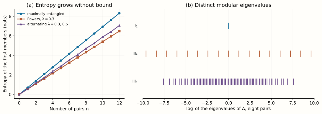
Thus the statement “infinitely many entangled pairs” does not specify an algebra. The same divergent entropy is compatible with types II${}_1$, III${}_{\lambda }$ and III${}_1$, and what distinguishes them here is the modular spectrum of the product state. These are algebraic models; they are not discretizations whose geometry has been shown to converge to a field theory.

5.3 Self-study: why one modular spectrum does not classify

The infinite-product examples might suggest that the modular spectrum of one state decides the type. But Lecture 3 exhibited a thermofield-double state of an oscillator pair with $\Delta |n,m⟩=q^{n-m}|n,m⟩$. Its modular spectrum is the closure of $\{q^k:k\in \mathbb{Z}\}$, exactly the ladder of the Powers factor with $\lambda =q$, and the algebra is the type-I algebra $\mathcal{B}({\ell }^2)$. Other faithful states give other unbounded spectra on the same algebra (Problem 8). The invariant that classifies factors is an intersection over states,

$$S(\mathcal{M})=\bigcap _{\phi }\mathrm{Sp}{\Delta }_{\phi },$$

where $\phi$ runs over faithful normal semifinite weights. It equals $\{1\}$ for semifinite factors, $\{0\}\cup {\lambda }^{\mathbb{Z}}$ for type III${}_{\lambda }$, and $[0,\infty )$ for type III${}_1$. For the infinite products above, the product state has enough symmetry that its spectrum computes the invariant; this is part of the Araki–Woods and Connes theorems.

For relativistic field theories the classification is a theorem with hypotheses. Araki showed in 1964 that the local algebras of the free field are of type III. Under a phase-space nuclearity condition and a short-distance scaling hypothesis, the local algebra of a bounded region with nonempty causal complement is isomorphic to the unique hyperfinite factor of type III${}_1$, possibly tensored with its center. [Stated only — refs: Fredenhagen 1985; Buchholz–D’Antoni–Fredenhagen 1987; AQFT Week 12, Theorem 1.1.] Lecture 10 identifies the vacuum modular operator of a wedge with a boost, whose spectrum is all of $(0,\infty )$; by the remark above this identification is an important input, and the classification requires separate arguments: for wedges it is Driessler’s theorem, and for bounded regions the results cited above (AQFT Week 12, §§2.3 and 5.1).

6. Relative entropy survives the loss of a trace

6.1 Araki’s definition

Let $\mathcal{M}$ act on $\mathcal{H}$ with two faithful normal states $\rho$ and $\sigma$, represented by vectors ${\xi }_{\rho }$ and ${\xi }_{\sigma }$. Generalizing the Tomita map of Lecture 3, written $S_T$ there and $S_{\Omega }$ here, the relative Tomita operator is defined on $\mathcal{M}{\xi }_{\rho }$ by

$$S_{\sigma |\rho }(A{\xi }_{\rho })=A^{†}{\xi }_{\sigma },{\Delta }_{\sigma |\rho }=S_{\sigma |\rho }^{†}\overline{S_{\sigma |\rho }},$$

and Araki’s relative entropy is

$$D_{\mathcal{M}}(\rho \Vert \sigma )=-⟨{\xi }_{\rho },\log {\Delta }_{\sigma |\rho }{\xi }_{\rho }⟩,$$

understood as $+\infty$ when ${\xi }_{\rho }$ is outside the appropriate domain. It depends only on the two states, and not on the vectors chosen to represent them. [Stated only — refs: Araki 1976; Witten §3.3.]

The definition reduces to the familiar one in finite dimensions. Represent $M_n$ on the Hilbert–Schmidt space of $n\times n$ matrices, by left multiplication, with ${\xi }_{\rho }={\rho }^{1/2}$ and ${\xi }_{\sigma }={\sigma }^{1/2}$. Writing $X=A{\rho }^{1/2}$, the relative Tomita operator is $S_{\sigma |\rho }(X)={\rho }^{-1/2}{X}^{†}{\sigma }^{1/2}$, which is $J{\Delta }^{1/2}$ with $J(X)=X^{†}$ and

$${\Delta }_{\sigma |\rho }(X)=\sigma X{\rho }^{-1}.$$

Left and right multiplications commute, so $\log {\Delta }_{\sigma |\rho }=L_{\log \sigma }-R_{\log \rho }$, and

$$D(\rho \Vert \sigma )=-\mathrm{Tr}{\rho }^{1/2}(\log \sigma ){\rho }^{1/2}+\mathrm{Tr}{\rho }^{1/2}{\rho }^{1/2}\log \rho =\mathrm{Tr}\rho (\log \rho -\log \sigma ).$$

This fixes the order of the two states and the sign. The general definition does not subtract two infinite von Neumann entropies, and it is finite for many pairs of states on type-III algebras.

6.2 Unitary excitations and modular energy

A class of states for which the relative entropy is explicit consists of those obtained from the vacuum by a unitary operator of the region itself.

Proposition. Proved, up to domain questions. Let $\Omega$ be cyclic and separating for $\mathcal{M}$, let $u\in \mathcal{M}$ be unitary, and let ${\omega }_u$ be the state of $u\Omega$ on $\mathcal{M}$. Then ${\Delta }_{\Omega |u\Omega }={\Delta }_{\Omega }$, and

$$D_{\mathcal{M}}({\omega }_u\Vert \omega )=⟨u\Omega ,\hat{K}u\Omega ⟩,\hat{K}=-\log {\Delta }_{\Omega }.$$

Proof. Take ${\xi }_{\rho }=u\Omega$ and ${\xi }_{\sigma }=\Omega$. For $A\in \mathcal{M}$ put $B=Au\in \mathcal{M}$, so that $A^{†}=u{B}^{†}$. Then $S_{\Omega |u\Omega }(B\Omega )=u{B}^{†}\Omega =u{S}_{\Omega }(B\Omega )$. Therefore $S_{\Omega |u\Omega }=u{S}_{\Omega }$, and since $u^{†}u=I$, ${\Delta }_{\Omega |u\Omega }=S_{\Omega }^{†}{u}^{†}u{S}_{\Omega }={\Delta }_{\Omega }$. Inserting this in the definition gives the formula. $\square$

The operator $\hat{K}$ is the full modular Hamiltonian of Lecture 3, and it annihilates $\Omega$. In finite dimensions the formula reads $D(u\sigma u^{†}\Vert \sigma )=\mathrm{Tr}(u\sigma u^{†}{K}_{\sigma })-\mathrm{Tr}(\sigma K_{\sigma })$ with $K_{\sigma }=-\log \sigma$: the entropy does not change under a unitary of the region, and the relative entropy is the change in the expectation value of the one-sided modular Hamiltonian. The displaced Gaussian states of Lecture 8, §4.3, are the lattice example, with $u$ a Weyl operator of the region. In the continuum the one-sided modular Hamiltonian does not exist as an operator, but the right-hand side above does. Lecture 10 evaluates it for the Rindler wedge and a coherent state, where $\hat{K}$ is $2\pi$ times the boost generator.

6.3 Properties used later

The relative entropy is nonnegative and vanishes only when the two states coincide. It decreases under restriction to a subalgebra: if $\mathcal{N}\subset \mathcal{M}$, then $D_{\mathcal{N}}(\rho {|}_{\mathcal{N}}\Vert \sigma {|}_{\mathcal{N}})\le D_{\mathcal{M}}(\rho \Vert \sigma )$, and more generally under completely positive unital maps. It is jointly convex and lower semicontinuous, and it can be infinite. [Stated only — refs: Araki 1976; Uhlmann 1977; Witten §§3.4–3.6.] In a field theory, monotonicity says that the distinguishability of two states can only grow with the region: if $O_1\subset O_2$, then $D_{\mathcal{A}(O_1)}\le D_{\mathcal{A}(O_2)}$. Lecture 20 uses monotonicity to bound recovery, and Lecture 21 identifies boundary and bulk relative entropies.

7. A buffer restores a tensor product

7.1 Split inclusions

Suppose $\overline{O_1}\subset O_2$, so that a buffer of finite size separates the boundary of $O_1$ from that of $O_2$. The inclusion $\mathcal{A}(O_1)\subset \mathcal{A}(O_2)$ is split if there is a type-I factor $\mathcal{N}$ with

$$\mathcal{A}(O_1)\subset \mathcal{N}\subset \mathcal{A}(O_2).$$

A type-I factor has a tensor-product form: there is a unitary identification $\mathcal{H}\simeq {\mathcal{H}}_1\otimes {\mathcal{H}}_2$ under which $\mathcal{N}=\mathcal{B}({\mathcal{H}}_1)\otimes I$ and ${\mathcal{N}}^{\prime }=I\otimes \mathcal{B}({\mathcal{H}}_2)$. Taking commutants reverses the second inclusion, $\mathcal{A}(O_2{)}^{\prime }\subset {\mathcal{N}}^{\prime }$. Therefore the inner region acts on the first factor and the exterior of the larger region on the second,

$$\mathcal{A}(O_1)\subset \mathcal{B}({\mathcal{H}}_1)\otimes I,\mathcal{A}(O_2{)}^{\prime }\subset I\otimes \mathcal{B}({\mathcal{H}}_2).$$

It follows that any normal states ${\phi }_1$ of $\mathcal{A}(O_1)$ and ${\phi }_2$ of $\mathcal{A}(O_2{)}^{\prime }$ extend to a normal product state $\phi (AB)={\phi }_1(A){\phi }_2(B)$: extend each to a normal state of its type-I factor, where it has a density matrix, and take the tensor product. This is statistical independence across the buffer. Note that the intermediate factor is not unique, and its tensor boundary lies somewhere in the buffer, so an entropy computed from it depends on the choice and is not a canonical entropy of the sharp region $O_1$.

Checkpoint 2. Does the split property turn $\mathcal{A}(O_1)$ into a type-I algebra?

Answer. No. A type-III algebra can sit inside a type-I factor, as any algebra of restricted observables sits inside $\mathcal{B}(\mathcal{H})$. The factor $\mathcal{N}$ is larger than $\mathcal{A}(O_1)$, and it contains observables of the buffer.

7.2 When the split property holds

For the free scalar field of positive mass the split property holds for every pair of regions separated by a buffer of positive size. In general it follows from nuclearity conditions, which bound the number of linearly independent local states of bounded energy. [Stated only — refs: Buchholz 1974; Buchholz–Wichmann 1986; Doplicher–Longo 1984; Fewster 2016.] It fails for touching regions. If $O_2$ shrinks to $O_1$ and Haag duality holds, the only algebra between $\mathcal{A}(O_1)$ and $\mathcal{A}(O_1^{\prime }{)}^{\prime }=\mathcal{A}(O_1)$ is $\mathcal{A}(O_1)$ itself, which is not type I, and there is no normal product state across the common boundary. Witten’s Section 7 gives an elementary account of the factorized states that the split property provides.

7.3 Finite correlations across a buffer

The split property explains the lattice experiment of Lecture 8. The mutual information of two separated intervals converged as the lattice was refined, while the entropy of each diverged. Hollands and Sanders make the continuum statement precise: with a corridor of positive width between two regions, entanglement measures such as the relative entropy of entanglement, the minimum of $D$ over separable normal states, are finite in free field theories and obey explicit upper and lower bounds, which typically diverge as the corridor closes and decay when the regions are far apart. This is the counterpart of the statement recorded in Lecture 8, Problem 14, that the lattice mutual information of adjacent intervals diverges as $a\to 0$.

Physical picture: the buffer. A sharp boundary severs correlations at every scale, and the lattice showed that there are infinitely many of them. A buffer of finite width leaves the correlations at scales shorter than its width inside the buffer, where neither party has access. What remains between the inner region and the far exterior is finite in the sense made precise by nuclearity. The width of the buffer then plays the role of the cutoff, and entropies computed with a split factor depend on it, as the lattice entropies depended on $a$.

8. What to take away

• Proved: given Reeh–Schlieder, the vacuum is separating for every region with a nonempty causal complement, so every local algebra carries a vacuum modular operator; local instruments cannot signal, and in a finite model preparing a rare Schmidt component costs an operator norm $p_j^{-1/2}$.
• Sketched: the Reeh–Schlieder theorem follows from the spectrum condition through analytic continuation of translated matrix elements; the analytic steps are only sketched, here and in AQFT Week 9.
• Exact calculation: infinite products with entropy $n\log 2$ or $nh(\lambda )$ have modular spectra $\{1\}$ or ${\lambda }^{\mathbb{Z}}$; the classification of the resulting factors as II${}_1$ and III${}_{\lambda }$ is stated with references, and divergent entropy alone does not decide the type.
• Proved: Araki’s relative entropy reduces to $\mathrm{Tr}\rho (\log \rho -\log \sigma )$ in finite dimensions, and for a unitary excitation by $u\in \mathcal{M}$ it equals $⟨u\Omega ,\hat{K}u\Omega ⟩$.
• Hypothesis-explicit: local algebras are of type III${}_1$ under nuclearity and scaling hypotheses, and inclusions with a buffer are split under nuclearity; the split factor gives product states and finite correlation measures, and depends on the buffer.

9. Looking ahead

Lecture 10 computes the modular operator of the vacuum for a Rindler wedge, where the Bisognano–Wichmann theorem identifies it with a boost, and evaluates the unitary-excitation formula of §6.2 for a coherent state; the answer is $2\pi$ times the boost energy of the classical wave, and the lattice of Lecture 8 approaches it. Lecture 11 transports the result to a ball in a conformal field theory. Lectures 20 and 21 use the relative entropy of §6 with monotonicity, and Lectures 28–30 return to nets, duality and inclusions of algebras.

10. Problem set

Classroom core

1. Separating from locality. Identify exactly where boundedness enters the proof of §4.3, and explain what would be needed for an unbounded field operator.

2. Postselection. For $\sqrt{p}|00⟩+\sqrt{1-p}|11⟩$ and the local projector $|0⟩⟨0|$ on the first qubit, find the conditional state of the second qubit, the probability of success, and the unconditional state after the measurement.

3. A finite relative modular operator. For diagonal $\rho =\mathrm{diag}(p_i)$ and $\sigma =\mathrm{diag}(q_i)$, compute the action of ${\Delta }_{\sigma |\rho }$ on the matrix units $E_{ij}$ and recover $D(\rho \Vert \sigma )={\sum }_i{p}_i\log (p_i/q_i)$.

4. Weyl operators and locality. Derive $W(f)W(g)W(f{)}^{†}=e^{-i\sigma (f,g)}W(g)$ from the Weyl relation, and conclude that Weyl operators with spacelike separated supports commute.

5. A Powers spectrum. For two Powers pairs with ratio $\lambda$, list the eigenvalues of ${\Delta }_2$ with their multiplicities, and check that the multiplicities add up to $16$.

6. The price of a rare component. In the finite model of §4.1, show that the smallest norm of an operator $A$ with $(A\otimes I)\Omega =e_k\otimes e_j$ is $p_j^{-1/2}$, and that a local instrument can produce $e_k\otimes e_j$ with probability at most $p_j$.

Self-study consolidation

7. An invalid inference. Criticize the argument: “the entropy diverges as the cutoff is removed; therefore the local algebra is of type III${}_1$.”

8. Type I with an unbounded modular operator. For the faithful state $p_n\propto e^{-n^2}$ on $\mathcal{B}({\ell }^2)$, compute the eigenvalues of $\Delta$ on matrix units and show that $\log \Delta$ is unbounded above and below.

9. Product states across a buffer. Explain why the tensor factors of a split inclusion concern $\mathcal{A}(O_1)$ and $\mathcal{A}(O_2{)}^{\prime }$, and why they do not give a tensor decomposition between $\mathcal{A}(O_1)$ and $\mathcal{A}(O_2)$.

10. Unitary excitations in finite dimensions. In the Hilbert–Schmidt representation, verify $D(u\sigma u^{†}\Vert \sigma )=⟨u{\sigma }^{1/2},\hat{K}u{\sigma }^{1/2}⟩$ with $\hat{K}=-\log {\Delta }_{\sigma }$, for $\sigma$ of full rank and $u$ unitary.

11. The quasifree vacuum. Derive $\omega (W(f))=e^{-\Vert f{\Vert }^2/2}$ from $\varphi (f)=a({\bar{f}}_{+})+a^{†}(f_{+})$, schematically, and show that $\omega (W(f)W(g))=e^{-i\sigma (f,g)/2}{e}^{-\Vert f+g{\Vert }^2/2}$.

12. Two ratios. Show that if $\alpha =\log {\lambda }_1/\log {\lambda }_2$ is irrational, then $\{k_1\log {\lambda }_1+k_2\log {\lambda }_2:k_1,k_2\in \mathbb{Z}\}$ is dense in $\mathbb{R}$.

Research extension

13. Correlations across a corridor. For a free massive scalar in $1+1$ dimensions, compute on the lattice the mutual information of two intervals separated by a corridor of width $d$, and compare it with the bounds of Hollands and Sanders for the relative entropy of entanglement. Known: both quantities are finite for $d>0$ and grow as $d\to 0$; since ${\rho }_A\otimes {\rho }_B$ is separable, the mutual information is an upper bound for the relative entropy of entanglement. Completion: the continuum values of $I$ as a function of $d$, with the lattice errors of Lecture 8 controlled, and a statement of which bound they test.

14. A detector test of the buffer. Two detectors, localized in $O_1$ and in the causal complement of $O_2$, couple to a free field in its vacuum. Formulate a protocol that estimates their correlation, with finite switching times and finite errors, and determine how it depends on the buffer. Known: for complementary wedges the vacuum violates the Bell inequalities maximally (Summers–Werner; AQFT Week 11); with a buffer the correlations decay, exponentially in a massive theory, and the Bell supremum can decrease. Completion: the leading-order correlation of the two detectors as a function of the separation, and the statement of what it does and does not establish about the algebras.

15. The scaling route to type III${}_1$. Reconstruct the logical structure of the argument that local algebras are of type III${}_1$. Known: Fredenhagen’s theorem under asymptotic scale invariance, and the scaling algebras of Buchholz and Verch, summarized in AQFT Week 12. Completion: a written account of how a scaling limit supplies a continuum of modular scales, with each hypothesis identified and the step at which the Connes invariant is computed.

11. Answer checkpoints

1. The vectors $B\Omega$ with $B\in \mathcal{A}(O^{\prime })$ are dense, and $A$ vanishes on them. A bounded operator is continuous, so it vanishes on the closure, which is $\mathcal{H}$. An unbounded operator can vanish on a dense domain and still be nonzero elsewhere, so one would need a common core and closability arguments.

2. Conditional on success the second qubit is $|0⟩$, and success has probability $p$. Averaging over both outcomes gives $p|0⟩⟨0|+(1-p)|1⟩⟨1|$ for the second qubit, its state before the measurement.

3. ${\Delta }_{\sigma |\rho }{E}_{ij}=\sigma E_{ij}{\rho }^{-1}=(q_i/p_j)E_{ij}$. With ${\xi }_{\rho }={\sum }_i\sqrt{p_i}{E}_{ii}$ only the diagonal matrix units contribute, and $-{\sum }_i{p}_i\log (q_i/p_i)={\sum }_i{p}_i\log (p_i/q_i)$.

4. Using the Weyl relation twice, $W(f)W(g)W(-f)=e^{-i\sigma (f,g)/2}W(f+g)W(-f)=e^{-i\sigma (f,g)/2}{e}^{-i\sigma (f+g,-f)/2}W(g)$, and $\sigma (f+g,-f)=\sigma (f,g)$ by antisymmetry. Spacelike supports give $\sigma =0$ because the Pauli–Jordan distribution vanishes there.

5. The reduced state has eigenvalues $1,\lambda ,\lambda ,{\lambda }^2$ up to normalization. The sixteen ratios $p_I/p_J$ give ${\lambda }^0$ six times, ${\lambda }^{\pm 1}$ four times each, and ${\lambda }^{\pm 2}$ once each: $6+4+4+1+1=16$.

6. $(A\otimes I)\Omega ={\sum }_i\sqrt{p_i}A{e}_i\otimes e_i=e_k\otimes e_j$ requires $A{e}_j=p_j^{-1/2}{e}_k$ and $A{e}_i=0$ for $i\ne j$, so $\Vert A\Vert \ge p_j^{-1/2}$, with equality for $p_j^{-1/2}{E}_{kj}$. A Kraus operator $M$ has $\Vert M\Vert \le 1$, and if $M\Omega$ is proportional to $e_k\otimes e_j$ then $M\Omega =\sqrt{p_j}M{e}_j\otimes e_j$, whose squared norm is at most $p_j$.

7. The tracial infinite product has divergent entropy and type II${}_1$, and the Powers products have divergent entropy and type III${}_{\lambda }$ with $\lambda <1$. Divergence of a regulated entropy decides neither type III nor its subtype; the classification uses the Connes invariant.

8. $\Delta E_{mn}=(p_m/p_n)E_{mn}=e^{-(m^2-n^2)}{E}_{mn}$, and $m^2-n^2$ takes arbitrarily large values of both signs. The algebra is $\mathcal{B}({\ell }^2)$, which is type I.

9. The inclusion $\mathcal{N}\subset \mathcal{A}(O_2)$ gives $\mathcal{A}(O_2{)}^{\prime }\subset {\mathcal{N}}^{\prime }$ by taking commutants. The tensor decomposition is between $\mathcal{N}$ and ${\mathcal{N}}^{\prime }$, and therefore between $\mathcal{A}(O_1)$ and $\mathcal{A}(O_2{)}^{\prime }$. The algebras $\mathcal{A}(O_1)$ and $\mathcal{A}(O_2)$ overlap, since the first is contained in the second.

10. With ${\Delta }_{\sigma }=L_{\sigma }{R}_{{\sigma }^{-1}}$, $\hat{K}=L_{K_{\sigma }}-R_{K_{\sigma }}$ with $K_{\sigma }=-\log \sigma$. Then $⟨u{\sigma }^{1/2},\hat{K}u{\sigma }^{1/2}⟩=\mathrm{Tr}({\sigma }^{1/2}{u}^{†}{K}_{\sigma }u{\sigma }^{1/2})-\mathrm{Tr}({\sigma }^{1/2}{u}^{†}u{\sigma }^{1/2}{K}_{\sigma })=\mathrm{Tr}(u\sigma u^{†}{K}_{\sigma })-\mathrm{Tr}(\sigma K_{\sigma })$, which is $D(u\sigma u^{†}\Vert \sigma )$ because $S(u\sigma u^{†})=S(\sigma )$.

11. For $X=i{a}^{†}(f_{+})$ and $Y=ia({\bar{f}}_{+})$, $e^{X+Y}=e^X{e}^Y{e}^{-[X,Y]/2}$ with $[X,Y]=\Vert f{\Vert }^2$. The vacuum expectation value of $e^X{e}^Y$ is one, since $a$ annihilates the vacuum on the right and $a^{†}$ on the left. The second formula follows from the Weyl relation.

12. The subgroup $\{k_1\alpha +k_2\}$ of $\mathbb{R}$ is dense when $\alpha$ is irrational, since a closed proper subgroup of $\mathbb{R}$ is cyclic, and a cyclic group cannot contain both $1$ and an irrational number. Multiplying by $\log {\lambda }_2$ gives the statement.

Wiki connections. Haag–Kastler axioms · Reeh–Schlieder theorem · Weyl operators · type III₁ von Neumann algebras · Araki–Uhlmann relative entropy