Lecture 10 — Rindler observers and modular time

Lecture 3 associated a flow with a state and an algebra, and Lecture 9 showed that every local algebra of a relativistic theory carries one. Here we meet the first case in which that flow moves observables through spacetime. For the vacuum restricted to a Rindler wedge, the Bisognano–Wichmann theorem identifies the modular flow with the boost that preserves the wedge, at rapidity $2\pi$ per unit of modular time. We keep three clocks apart, the modular parameter, the rapidity and the proper time of an accelerated observer, and convert between them. The factor $2\pi$ is then checked three times: in the analytic structure of the vacuum two-point function along an accelerated orbit, in the response of a detector, and in the Bogoliubov coefficients of Unruh’s modes. Finally the unitary-excitation formula of Lecture 9 gives the relative entropy of a coherent state as $2\pi$ times the boost energy of a classical wave, and the lattice of Lecture 8 approaches that value.

How to use this lecture

Classroom core, two meetings of two hours. The first meeting covers the history (§1, 10 minutes), the wedge and its accelerated observers (§2, 25 minutes), the Bisognano–Wichmann theorem and the three clocks (§§3.1–3.3, 35 minutes), and the KMS condition along an orbit (§4, 35 minutes), leaving 15 minutes for Checkpoint 1 and Problem 1. The second meeting covers the detector (§5, 35 minutes), Unruh’s modes (§6, 30 minutes), and the relative entropy of a coherent state (§§7.1–7.2, 35 minutes), with 20 minutes for Checkpoint 2 and Problem 3; Problems 2 and 4–6 complete the core assignment. These allocations are proposals and have not been tested in class.

Self-study. The Euclidean origin of $2\pi$ and Takesaki’s uniqueness argument (§3.4), the lattice test of the coherent-state formula (§7.3), temperature and redshift near a horizon (§8), and Problems 7–12.

Research extension. Finite switching times, the quantum null energy condition for coherent states, and the continuum limit of the lattice test, in Problems 13–15.

Prerequisites. Lecture 3 for the modular flow ${\sigma }_s(A)={\Delta }^{-is}A{\Delta }^{is}$ and the upper-strip KMS condition; Lecture 8 for the lattice modular Hamiltonian and the relative entropy of a displaced Gaussian state; Lecture 9 for local algebras, Weyl operators and the unitary-excitation formula. Special relativity and contour integration.

What this lecture establishes. The Bisognano–Wichmann theorem is stated with its hypotheses, as in AQFT Week 10; its proof is in the papers of Bisognano and Wichmann and in the modern account of Borchers. The Rindler kinematics, the KMS property of the two-point function along an orbit, the detector response and the Bogoliubov ratio are exact calculations for free fields. The coherent-state relative entropy is derived from Lecture 9 and the theorem, with domain questions left to the rigorous treatments of Longo and of Casini, Grillo and Pontello, and it is tested numerically on the lattice.

0. Reading

Primary.

• J. J. Bisognano, E. H. Wichmann, On the duality condition for a Hermitian scalar field, J. Math. Phys. 16 (1975) 985, and On the duality condition for quantum fields, J. Math. Phys. 17 (1976) 303.
• W. G. Unruh, Notes on black-hole evaporation, Phys. Rev. D 14 (1976) 870.
• E. Witten, Notes on Some Entanglement Properties of Quantum Field Theory (2018), Section 5.
• AQFT course, Week 10.

Secondary.

• L. C. B. Crispino, A. Higuchi, G. E. A. Matsas, The Unruh effect and its applications (2007).
• G. L. Sewell, Quantum fields on manifolds: PCT and gravitationally induced thermal states, Ann. Phys. 141 (1982) 201.
• H.-J. Borchers, On revolutionizing quantum field theory with Tomita’s modular theory, J. Math. Phys. 41 (2000) 3604.
• B. S. DeWitt, Quantum gravity: the new synthesis, in S. W. Hawking and W. Israel (eds.), General Relativity: An Einstein Centenary Survey (Cambridge University Press, 1979).
• S. A. Fulling, Nonuniqueness of canonical field quantization in Riemannian space-time, Phys. Rev. D 7 (1973) 2850; P. C. W. Davies, Scalar production in Schwarzschild and Rindler metrics, J. Phys. A 8 (1975) 609.
• W. G. Unruh, R. M. Wald, What happens when an accelerating observer detects a Rindler particle, Phys. Rev. D 29 (1984) 1047.

Optional research reading.

• R. Longo, Entropy of Coherent Excitations (2019).
• H. Casini, S. Grillo, D. Pontello, Relative entropy for coherent states from Araki formula (2019).
• F. Ciolli, R. Longo, G. Ruzzi, The information in a wave (2019).
• H. Casini, E. Teste, G. Torroba, Modular Hamiltonians on the null plane and the Markov property of the vacuum state (2017).
• H. Casini, Relative entropy and the Bekenstein bound (2008).
• S. Takagi, Vacuum noise and stress induced by uniform acceleration, Prog. Theor. Phys. Suppl. 88 (1986) 1.
• W. Driessler, On the type of local algebras in quantum field theory, Commun. Math. Phys. 53 (1977) 295.

1. Three discoveries of one temperature

In 1973 Fulling observed that quantizing a free field in the coordinates adapted to a uniformly accelerated observer gives a notion of particle, and a vacuum, different from the inertial ones. Two years later Davies found a thermal spectrum in the same setting, and in 1976 Unruh gave the result its operational form. Motivated by Hawking’s discovery of black-hole radiation, Unruh coupled a model detector, a particle in a box with discrete levels, to the field and showed that a detector with proper acceleration $a$, moving through the Minkowski vacuum, is excited as if it were immersed in a thermal bath at temperature $a/2\pi$. DeWitt reduced the model in 1979 to the point-like two-level system that we use in §5.

At the same time, and for entirely different reasons, Bisognano and Wichmann were studying the duality condition of axiomatic field theory, the statement that the commutant of a wedge algebra is the algebra of the opposite wedge. In 1975 and 1976 they proved that the modular operator of the vacuum for a wedge algebra is $e^{-2\pi K}$, with $K$ the generator of the boosts that preserve the wedge. In 1982 Sewell showed that the two results are the same result: the theorem of Bisognano and Wichmann is the Unruh effect stated as a KMS condition, and it extends to spacetimes with bifurcate Killing horizons, where it describes Hawking radiation. Unruh and Wald clarified in 1984 what the inertial observer sees when the accelerated detector clicks: the detector emits a quantum.

This lecture follows the theorem and checks it by hand. For the course, the wedge is the first example of a modular flow with a geometric meaning, and every geometric modular flow of later lectures descends from it: the ball of Lecture 11 by a conformal map, the entanglement wedges of Lectures 19–21 by the holographic dictionary, and the emergent times of Lecture 31 by modular inclusions.

2. The wedge and its accelerated observers

In Minkowski coordinates $(t,x,\mathbf{y})$ in $d$ spacetime dimensions, with $\mathbf{y}$ the $d-2$ transverse coordinates, take the right wedge $W_R=\{x>|t|\}$ and write

$$t=\xi \sinh \eta ,x=\xi \cosh \eta ,\xi >0,\eta \in \mathbb{R}.$$

Direct differentiation gives the Rindler metric

$$d{s}^2=-{\xi }^{2}d{\eta }^2+d{\xi }^2+d{\mathbf{y}}^2.$$

A trajectory at fixed $\xi$ and $\mathbf{y}$ has proper time $\tau =\xi \eta$, velocity $u=(\cosh (\tau /\xi ),\sinh (\tau /\xi ))$ in the $(t,x)$ plane, and acceleration $du/d\tau =(\sinh (\tau /\xi ),\cosh (\tau /\xi ))/\xi$, of Minkowski norm $1/{\xi }^2$. The proper acceleration is therefore $a=1/\xi$. The null planes $x=\pm t$ bound the wedge and are the horizons of these observers: no signal sent from an event with $t\ge x$ ever reaches their orbits, and no signal sent from the orbits reaches an event with $t\le -x$.

The boosts in the $(t,x)$ plane translate $\eta$ and preserve the wedge, each orbit and the value of $\xi$. Their Killing vector is $\chi =x{\partial }_t+t{\partial }_x={\partial }_{\eta }$, future directed in $W_R$ and past directed in the left wedge $W_L=\{x<-|t|\}$. We fix the implementer convention of AQFT Week 10,

$$U(\Lambda (\eta ))=e^{i\eta K},K=\int d^{d-1}xx{T}_{00}(0,x,\mathbf{y}),$$

where the integral runs over the whole slice $t=0$. The weight $x$ is positive on the right and negative on the left, so $K$ generates future-directed evolution on the right and past-directed evolution on the left. The vacuum is invariant, $K\Omega =0$, and $K$ has spectrum $\mathbb{R}$. The causal complement of $W_R$ is $W_L$. The stress-tensor expression is formal: the theorem below uses only the self-adjoint generator of the unitary boost representation.

3. The Bisognano–Wichmann theorem

3.1 The sign convention

The course convention, shared with the AQFT course, is

$${\sigma }_s(A)={\Delta }^{-is}A{\Delta }^{is}.$$

For a matrix state $\rho =e^{-K_{\rho }}/Z$ in the representation of Lecture 3 this becomes ${\sigma }_s(A)=e^{is{K}_{\rho }}A{e}^{-is{K}_{\rho }}$ on the accessible algebra, the Heisenberg evolution generated by $K_{\rho }$. The KMS condition at unit inverse temperature reads, for suitable $A$ and $B$,

$$F_{AB}(s)=\omega (A{\sigma }_s(B)),F_{AB}(s+i)=\omega ({\sigma }_s(B)A),$$

with $F_{AB}$ analytic in the strip $0<\mathrm{Im}s<1$. The more common mathematical convention ${\Delta }^{it}A{\Delta }^{-it}$ corresponds to $t=-s$.

3.2 The theorem

Theorem (Bisognano–Wichmann, 1975–76). Stated only — refs: Bisognano–Wichmann; Borchers 2000; AQFT Week 10, Theorem 1.1. Consider a Wightman theory of finitely many Hermitian fields satisfying Poincaré covariance, the spectrum condition, locality and cyclicity of the vacuum, and suppose that the von Neumann algebras generated by the fields smeared in spacelike separated regions commute. Let $\mathcal{A}(W_R)$ be the von Neumann algebra generated by the fields smeared in $W_R$. Then the vacuum modular operator and conjugation of $\mathcal{A}(W_R)$ are

$${\Delta }_{W_R}=e^{-2\pi K},J_{W_R}={\Theta }_W,$$

where ${\Theta }_W$ is the antiunitary operator that implements the reflection $(t,x,\mathbf{y})\mapsto (-t,-x,\mathbf{y})$ on the fields. In four dimensions ${\Theta }_W$ is the CPT operator composed with a rotation by $\pi$ in the transverse plane, and in two dimensions it is the CPT operator itself. For Fermi fields $J$ carries the statistics twist, and wedge duality below holds in its twisted form. In the convention of §3.1,

$${\sigma }_s(A)=U(\Lambda (2\pi s))AU(\Lambda (2\pi s){)}^{†}.$$

Two consequences are immediate. Tomita’s theorem gives $J\mathcal{A}(W_R)J=\mathcal{A}(W_R{)}^{\prime }$, and the geometric action of $J$ maps $W_R$ to $W_L$; therefore $\mathcal{A}(W_R{)}^{\prime }=\mathcal{A}(W_L)$, which is Haag duality for wedges. And the full modular Hamiltonian of Lecture 3 is $\hat{K}=-\log {\Delta }_{W_R}=2\pi K$, a two-sided operator. The regulated notation

$$K_R=2\pi {\int }_{x>0}{d}^{d-1}xx{T}_{00}(0,x,\mathbf{y})+\text{constant}$$

gives the action on right-wedge observables, and it is the continuum counterpart of the lattice modular Hamiltonian of a half-chain in Lecture 8. In the continuum it does not define the logarithm of a trace-class regional density matrix.

The theorem applies to every observable of the wedge, in every Wightman theory that satisfies these hypotheses, free or interacting. But it concerns the vacuum and the wedge: excited states, and bounded regions of a theory without conformal symmetry, generally have modular flows that are not induced by any spacetime transformation.

3.3 Three clocks

Three parameters now describe the same motion. The modular parameter $s$ is dimensionless and belongs to the state and the algebra. The rapidity $\eta =2\pi s$ is dimensionless and belongs to the boost. The proper time of the observer at $\xi$ is

$$\tau =\xi \eta =2\pi \xi s,$$

and it carries units of length. The conversion between modular and proper time depends on the trajectory. An imaginary modular shift $s\to s+i$, the KMS period, corresponds to $\tau \to \tau +2\pi i\xi$. The observer at $\xi$ therefore assigns to the vacuum the inverse temperature and temperature

$${\beta }_{\mathrm{proper}}=2\pi \xi =\frac{2\pi }{a},T_{\mathrm{proper}}=\frac{a}{2\pi },$$

or $k_{B}T=\hslash a/(2\pi c)$ in ordinary units. An acceleration of $10^{20}m/{\mathrm{s}}^2$ gives about $0.4\mathrm{K}$.

3.4 Self-study: why $2\pi$

Two arguments make the factor plausible before any calculation, and the first is Euclidean. Under $t=-i{t}_E$ the boost $\eta \mapsto \eta +\theta$ with imaginary rapidity $\theta =i\vartheta$ becomes a rotation by the angle $\vartheta$ in the $(t_E,x)$ plane, and the wedge becomes a half-plane. In the implementer convention, ${\Delta }^{1/2}=e^{-\pi K}=U(\Lambda (i\pi ))$ is the analytic boost through the angle $\pi$, which maps the right half-plane onto the left one, where $J$ takes over. A full turn has angle $2\pi$, and the vacuum correlation functions are single valued around it: this is the KMS period in rapidity. The half-chain of Lecture 8, whose reduced density matrix is a product of corner transfer matrices turning the lattice by a full angle, is the regulated version of the same picture. [Heuristic.]

The second argument uses Takesaki’s uniqueness theorem, AQFT Week 6, Theorem 2.2; Lecture 3 proves only its finite-dimensional counterpart, that a faithful state is KMS for its own modular flow. The theorem says that the modular flow is the unique one-parameter automorphism group for which a faithful normal state satisfies the KMS condition at unit inverse temperature. The vacuum is faithful on $\mathcal{A}(W_R)$ by Lecture 9, and the boosts preserve the wedge. If the boosts, rescaled by $2\pi$, satisfy the KMS condition, then they are the modular flow. What remains is to verify the KMS condition for all wedge observables, which requires the analytic continuation of Wightman functions in the rapidity; this is the content of the proof of Bisognano and Wichmann. [Sketched; AQFT Week 10, §2, lists the ingredients, and the proof is in Bisognano–Wichmann and in Borchers 2000.] Sections 4–6 check the KMS condition, and its consequences, for the free field.

4. The KMS condition along an accelerated orbit

For a free massless scalar in four spacetime dimensions the vacuum Wightman function is

$$G^{+}(x,x^{\prime })=⟨0|\varphi (x)\varphi (x^{\prime })|0⟩=-\frac{1}{4{\pi }^2}\frac{1}{(t-t^{\prime }-i0{)}^2-|\mathbf{x}-{\mathbf{x}}^{\prime }{|}^2}.$$

Restrict it to the orbit $t(\tau )=a^{-1}\sinh a\tau$, $x(\tau )=a^{-1}\cosh a\tau$. With $u=\tau -{\tau }^{\prime }$ and $v=(\tau +{\tau }^{\prime })/2$,

$$t-t^{\prime }=\frac{2}{a}\cosh (av)\sinh \frac{au}{2},x-x^{\prime }=\frac{2}{a}\sinh (av)\sinh \frac{au}{2},$$

so that $(t-t^{\prime }{)}^2-(x-x^{\prime }{)}^2=\frac{4}{a^2}{\sinh }^2\frac{au}{2}$. Since $t$ increases with $\tau$, the prescription $t-t^{\prime }-i0$ becomes $u-i0$, and

$$G^{+}(u)=-\frac{a^2}{16{\pi }^2}\frac{1}{{\sinh }^2\left[\frac{a}{2}(u-i0)\right]}.$$

The function depends only on $u$, because the orbit is a boost orbit and the vacuum is boost invariant. It is the boundary value from below, $u\to u-i0$, of the function $-\frac{a^2}{16{\pi }^2}{\sinh }^{-2}(az/2)$, which is analytic in the open strip $-2\pi /a<\mathrm{Im}z<0$ and has double poles at $z=2\pi in/a$; those at $n=0$ and $n=-1$ lie on the two edges of the strip.

Now take $A=B=\varphi (x(0))$, smeared along the orbit if one wishes to work with operators. The modular flow moves $B$ along the orbit by $u=2\pi s/a$, so that

$$F(s)=\omega (A{\sigma }_s(B))=⟨0|\varphi (x(0))\varphi (x(2\pi s/a))|0⟩=G^{+}\left(-\frac{2\pi s}{a}\right).$$

This is analytic for $0<\mathrm{Im}s<1$, which is the upper KMS strip. At its upper edge, using $\sinh (z-i\pi )=-\sinh z$,

$$F(s+i)=G^{+}\left(-\frac{2\pi s}{a}-\frac{2\pi i}{a}\right)=G^{+}\left(\frac{2\pi s}{a}\right)=\omega ({\sigma }_s(B)A).$$

The two-point function along the orbit therefore satisfies the KMS condition of §3.1 at unit modular inverse temperature, which is inverse proper temperature $2\pi /a$. [Exact calculation.] The theorem asserts the same for every pair of wedge observables; here we have verified it for the one correlation function that a detector on the orbit samples.

Checkpoint 1. Which geometric fact makes $G^{+}$ along the orbit a function of $u$ alone, and which analytic fact fixes the width of the strip?

Answer. The orbit is an orbit of a symmetry of the vacuum, so the correlation depends only on the boost separation. The width $2\pi /a$ is the distance between the pole at $u=0$ and the next pole at $u=-2\pi i/a$, the spacing of the zeros of $\sinh (au/2)$, which is the imaginary period of ${\sinh }^2(au/2)$.

5. A detector

Following DeWitt, we idealize the detector as a two-level system with levels $|g⟩$ and $|e⟩$ separated by a gap $E$, coupled along its worldline by

$$H_{\mathrm{int}}(\tau )=\lambda \chi (\tau )\mu (\tau )\varphi (x(\tau )),$$

where $\mu$ is the monopole operator of the detector, $\chi$ a switching function, and $\lambda$ a small coupling. At first order the probability of a transition from $|g⟩$ to $|e⟩$, summed over all final states of the field, is ${\lambda }^2|⟨e|\mu (0)|g⟩{|}^2\mathcal{F}(E)$, with

$$\mathcal{F}(E)=\int d\tau d{\tau }^{\prime }\chi (\tau )\chi ({\tau }^{\prime })e^{-iE(\tau -{\tau }^{\prime })}{G}^{+}(x(\tau ),x({\tau }^{\prime })).$$

The response function contains the field only through its two-point function on the worldline. For a stationary trajectory $G^{+}$ depends on $u=\tau -{\tau }^{\prime }$, and for switching times much longer than $1/E$ and $1/a$ the probability grows linearly with the duration, at the rate

$$\dot{\mathcal{F}}(E)={\int }_{-\infty }^{\infty }du{e}^{-iEu}{G}^{+}(u).$$

We evaluate it by shifting the contour to the middle of the analyticity strip of §4, $u=v-i\pi /a$. The shift is allowed because the integrand is analytic in the strip and decays as $|\mathrm{Re}u|\to \infty$. On the new contour $\sinh [\frac{a}{2}(v-i\pi /a)]=-i\cosh \frac{av}{2}$, so that

$$\dot{\mathcal{F}}(E)=e^{-\pi E/a}\frac{a^2}{16{\pi }^2}{\int }_{-\infty }^{\infty }dv\frac{e^{-iEv}}{{\cosh }^2(av/2)}=e^{-\pi E/a}\frac{a^2}{16{\pi }^2}\frac{4\pi E/a^2}{\sinh (\pi E/a)},$$

where we used $\int dx{e}^{-ikx}{\cosh }^{-2}x=\pi k/\sinh (\pi k/2)$. Therefore

$$\dot{\mathcal{F}}(E)=\frac{E}{2\pi }\frac{1}{e^{2\pi E/a}-1},\frac{\dot{\mathcal{F}}(E)}{\dot{\mathcal{F}}(-E)}=e^{-2\pi E/a}.$$

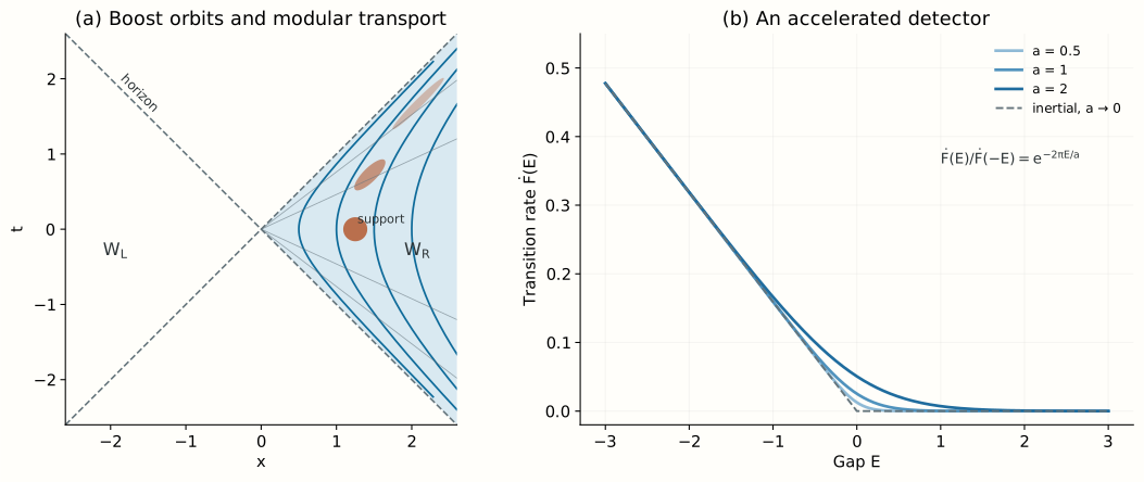
[Exact calculation.] Note that the integral over $v$ is even in $E$, so the whole asymmetry between excitation, $E>0$, and de-excitation, $E<0$, comes from the factor $e^{-\pi E/a}$ produced by the half-width of the strip. Detailed balance at temperature $a/2\pi$ is thus the KMS strip seen through a Fourier transform. For $a=1.3$ and $E=0.7$ the formula gives $\dot{\mathcal{F}}=3.9137\times 10^{-3}$, and a direct numerical integration along any line $\mathrm{Im}u=-\delta$ with $0<\delta <2\pi /a$ reproduces it, as Cauchy’s theorem requires. In the inertial limit $a\to 0$ at fixed $E>0$ the excitation rate vanishes as $e^{-2\pi E/a}$, while the de-excitation rate tends to $E/2\pi$, the spontaneous emission of the detector in this normalization.

The ratio of rates is the operational thermal statement. A detector left on long enough reaches the population $p_e/p_g=e^{-2\pi E/a}$, a two-level Gibbs state at temperature $a/2\pi$ (Problem 3), although the scalar field itself contributes a Planck factor. Note that no thermal bath is present. The field starts in the Minkowski vacuum, and in the inertial description each excitation of the detector is accompanied by the emission of a Minkowski quantum, with the energy supplied by the agent that keeps the detector accelerating.

Physical picture: a thermometer on a hyperbola. The detector reads the temperature of the correlations it samples, and those are the vacuum correlations along a boost orbit. They are thermal because the orbit is an orbit of the modular flow. An inertial detector samples correlations along a translation orbit, whose generator is positive, and it stays in its ground state. The same vacuum is thus cold for one observer and warm for another, with no contradiction, because the two observers measure different correlation functions. This is exact for the detector at leading order in $\lambda$ and at long times; finite switching adds transient terms (Problem 13).

6. Unruh’s modes

The same Planck factor appears in the mode expansion of the field, and Unruh’s derivation shows where it comes from. Take a massless field in two dimensions and its right-moving part ${\varphi }_R(x^{-})$, with $x^{\pm }=t\pm x$. Minkowski positive-frequency modes are $e^{-ik{x}^{-}}$ with $k>0$. They are boundary values of functions analytic and bounded in the lower half of the complex $x^{-}$ plane, and any such boundary value is a superposition of positive frequencies only.

In the right wedge $x^{-}=-\xi e^{-\eta }<0$, and the Rindler modes

$$(-x^{-}{)}^{i\omega }={\xi }^{i\omega }{e}^{-i\omega \eta },\omega >0,$$

are positive frequency with respect to $\eta$. In the left wedge $x^{-}>0$, and there the future-directed Rindler time runs opposite to $\eta$; the function $(x^{-}{)}^{i\omega }$ is the complex conjugate of a positive-frequency mode of the left wedge. Consider now the function $z^{i\omega }$ with its branch cut in the upper half-plane. It is analytic and bounded in the lower half-plane, and its boundary values on the real axis are

$$(x^{-}{)}^{i\omega }\text{for }{x}^{-}>0,e^{\pi \omega }(-x^{-}{)}^{i\omega }\text{for }{x}^{-}<0,$$

because the negative real axis is reached from below at $z=|x^{-}|e^{-i\pi }$. Therefore the combination

$$U_{\omega }=e^{\pi \omega /2}\theta (-x^{-})(-x^{-}{)}^{i\omega }+e^{-\pi \omega /2}\theta (x^{-})(x^{-}{)}^{i\omega }$$

is a Minkowski positive-frequency function, and its annihilation operator annihilates the Minkowski vacuum. In terms of the Rindler operators of the two wedges, that operator is proportional to $e^{\pi \omega /2}{b}_{\omega }^R-e^{-\pi \omega /2}(b_{\omega }^L{)}^{†}$; the relative sign comes from the negative Klein–Gordon norm of a conjugate mode. Normalized, it reads $d_{\omega }=\cosh r_{\omega }{b}_{\omega }^R-\sinh r_{\omega }(b_{\omega }^L{)}^{†}$ with

$$\tanh r_{\omega }=e^{-\pi \omega },\frac{|{\beta }_{\omega }{|}^2}{|{\alpha }_{\omega }{|}^2}={\tanh }^2{r}_{\omega }=e^{-2\pi \omega }.$$

From $d_{\omega }|0_M⟩=0$ and the analogous condition for the second Unruh combination one obtains

$$⟨0_M|(b_{\omega }^R{)}^{†}{b}_{\omega }^R|0_M⟩={\sinh }^2{r}_{\omega }=\frac{1}{e^{2\pi \omega }-1}$$

for a normalized wave packet of Rindler frequency near $\omega$. [Exact calculation, in the mode sense.] This is the Bose–Einstein distribution at inverse temperature $2\pi$ in the rapidity, that is, at proper temperature $a/2\pi$. AQFT Week 10, §4, obtains the same ratio from the Mellin transform ${\int }_0^{\infty }du{u}^{s-1}{e}^{iku}=\Gamma (s)e^{i\pi s/2}{k}^{-s}$.

The monodromy of $z^{i\omega }$ around the horizon point $x^{-}=0$, $|e^{i\omega \log (-1)}|=e^{\pi \omega }$ with the side fixed by positivity of the energy, is where the Boltzmann factor comes from. The regulated picture that goes with it writes the Minkowski vacuum as a thermofield double of the two wedges, ${\prod }_{\omega }{\sum }_n{e}^{-\pi \omega n}|n{⟩}_R|n{⟩}_L$ up to normalization. In the continuum this is formal: the touching wedge algebras do not define a tensor factorization of the Minkowski Hilbert space, as Lecture 9 explained, and the exact statement is the KMS condition of §§3–4.

7. The modular flow of a wave

7.1 Weyl operators

For a real test function $f$ supported in $W_R$, covariance and the theorem give

$${\sigma }_s(W(f))=W(f\circ \Lambda (-2\pi s)).$$

The modular flow acts on the test function by a boost, and on its support by $\mathrm{supp}f\mapsto \Lambda (2\pi s)\mathrm{supp}f$. This is the continuum form of the statement of Lecture 8 that the modular flow of a Gaussian state is a linear canonical transformation. The center of a bump moves along a hyperbola of fixed $\xi$, toward future null infinity as $s\to +\infty$ and toward past null infinity as $s\to -\infty$. It never approaches the edge of the wedge, which can be reached only by a separate sequence of supports with $\xi \to 0$.

7.2 The relative entropy of a coherent state

A coherent state is ${\psi }_f=W(f)\Omega$. Since $W(f)$ is a unitary of $\mathcal{A}(W_R)$ when $\mathrm{supp}f\subset W_R$, the proposition of Lecture 9, §6.2, applies with $\hat{K}=2\pi K$:

$$D_{\mathcal{A}(W_R)}({\omega }_f\Vert \omega )=⟨{\psi }_f,2\pi K{\psi }_f⟩.$$

The expectation value is computed from the action of $W(f)$ on the field. From $[\varphi (f),\varphi (x)]=i\int dyf(y)\Delta (y-x)$,

$$W(f{)}^{†}\varphi (x)W(f)=\varphi (x)+{\Phi }_f(x),{\Phi }_f(x)=\int dy\Delta (y-x)f(y),$$

where ${\Phi }_f$ is a classical solution of the Klein–Gordon equation. A normal-ordered stress tensor is quadratic in the field, so its expectation value in ${\psi }_f$ is the classical stress tensor of ${\Phi }_f$. The Cauchy data of ${\Phi }_f$ on $t=0$ lie in $x>0$, because they are determined by $f$ through causal propagation from $\mathrm{supp}f\subset W_R$. Therefore, using $K\Omega =0$,

$$D_{\mathcal{A}(W_R)}({\omega }_f\Vert \omega )=2\pi {\int }_{x>0}{d}^{d-1}xx\frac{1}{2}{\left[{\dot{\Phi }}_f^2+(\nabla {\Phi }_f{)}^2+m^2{\Phi }_f^2\right]}_{t=0}.$$

The relative entropy is $2\pi$ times the boost energy of the classical wave, the energy weighted by the distance from the edge. [Derived, with formal manipulation of $K$ on the coherent vectors; Stated only — refs: Longo 2019; Casini–Grillo–Pontello 2019, for the rigorous proofs.] Longo shows that the formula holds also for Cauchy data that cross the edge, with the integral restricted to $x>0$. Casini, Grillo and Pontello show that the canonical stress tensor is the one that appears, since an improvement term would add a contribution at the edge that violates positivity or monotonicity. The formula has the properties required of a relative entropy: it is nonnegative, and it decreases when the wedge is shrunk by a translation into itself, since both the region and the weight shrink.

For a packet whose energy $E$ is concentrated at distance $R$ from the edge, the formula gives $D\simeq 2\pi RE$. Casini proposed in 2008 that the positivity of this relative entropy, written as $\Delta S\le \Delta ⟨K_R⟩$ for regulated quantities, is the precise flat-space form of Bekenstein’s bound $S\le 2\pi RE$, and Lecture 11 obtains its analog for a ball.

Checkpoint 2. Why does the entropy of the coherent state not appear in the formula?

Answer. The state is obtained by a unitary of the region, and in finite dimensions such a unitary leaves the entropy unchanged, so the relative entropy is the change of the one-sided modular energy. In the continuum neither entropy is defined, but the right-hand side of Lecture 9, §6.2, is, and it reduces to the modular energy of the wave.

7.3 Self-study: a lattice test

The lattice of Lecture 8 tests the formula directly. For a displacement $\delta q$ of the lattice field, the relative entropy of the displaced vacuum restricted to a region is $\frac{1}{2}\delta q^{T}M\delta q$, with $M$ the kernel of the lattice modular Hamiltonian (Lecture 8, §4.3). Take $m=1$, a profile $\delta \varphi (x)=\exp [-(x-2{)}^2/(2\cdot 0.6^2)]$ with zero momentum, and the region $0<x<8$. To remove the second entangling point, the chain runs from $x=-8$ to $x=8$ between Dirichlet walls, so that the region has a single cut at $x=0$, where the profile is negligible, $\delta \varphi (0)\approx 0.004$. The continuum prediction is

$$D_{\mathrm{BW}}=2\pi {\int }_0^{\infty }dxx\frac{1}{2}\left(\delta {\varphi }^{\prime 2}+m^2\delta {\varphi }^2\right)=15.9626,$$

equal within $10^{-6}$ to $2\pi RE$ with $R=2$ and $E=1.2703$ the energy of the profile. The kernel $M$ requires high-precision arithmetic, for the reason given in Lecture 8, and the course script uses between 130 and 330 significant digits. The results are

$1/a$	lattice $D$	$D/D_{\mathrm{BW}}$
4	15.6976	0.98340
8	15.8903	0.99547
12	15.9264	0.99773

The deficits $1.66$, $0.45$ and $0.23$ percent are fitted to within $0.02$ percent by $0.26a^2+0.0005$, a discretization error of order $a^2$ on top of a small constant, and the extrapolation $a\to 0$ gives $0.9995$. The remaining $0.05$ percent is close to the difference, $0.04$ percent, between the wall at $x=8$ and a much longer interval at the same spacing. The course script scripts/lattice-coherent-entropy.py reproduces the table. An interval with two cuts approaches nearly the same value only when it is much longer than the packet: with $1/a=8$, intervals of length $8$, $12$, $16$ and $20$ give $0.9755$, $0.9936$, $0.9956$ and $0.9959$. [Numerical, in the lattice model; the extrapolation is not a proof of convergence.] The modular Hamiltonian of a half-line in the lattice vacuum thus approaches $2\pi$ times the boost generator in the sense tested here, through its position kernel on one smooth profile with zero momentum.

The figure summarizes the geometry of the lecture.

8. Self-study: temperature, redshift and horizons

Observers at different $\xi$ assign different temperatures to the same state, $T_{\mathrm{proper}}=1/(2\pi \xi )$. The product with the redshift factor $\sqrt{-g_{\eta \eta }}=\xi$ is constant,

$$T_{\mathrm{proper}}\sqrt{-g_{\eta \eta }}=\frac{1}{2\pi },$$

which is Tolman’s law for a system in equilibrium in a static gravitational field. The equivalence principle turns this into a statement about black holes. Near the horizon of the Schwarzschild solution, with $r=2M+{\rho }^2/8M$ at leading order, the metric becomes $-{\kappa }^2{\rho }^{2}d{t}^2+d{\rho }^2+(2M{)}^{2}d{\Omega }^2$ with surface gravity $\kappa =1/4M$. That is a Rindler metric with $\eta =\kappa t$. A static observer at small $\rho$ measures $T=1/(2\pi \rho )$, and redshifting to infinity gives $T_H=\kappa /2\pi =1/(8\pi M)$, Hawking’s temperature. [Heuristic here; Sewell 1982 and Kay–Wald 1991 give the theorem for bifurcate Killing horizons.] Lecture 23 uses the Euclidean form of this argument, regularity of the $(t_E,\rho )$ plane at $\rho =0$, which is the $2\pi$ of §3.4.

In odd spacetime dimensions the detector response of a scalar field contains a Fermi–Dirac factor instead of a Planck factor, although detailed balance at temperature $a/2\pi$ still holds. The KMS condition fixes the ratio of rates; the density of states of the field on the orbit fixes the rest. [Stated only — refs: Takagi 1986.]

9. What the wedge does and does not transfer

We have one controlled chain of statements. An algebra and a state determine a modular flow; the theorem identifies it, for the vacuum and a wedge, with a spacetime symmetry; and a trajectory converts the modular parameter into proper time. Later holographic arguments will have to supply each link. Lecture 11 obtains the first link and the second for a ball by conformal symmetry, and Lectures 18–22 ask when a bulk geometry supplies them for a boundary region.

The chain also marks its limits. A horizon alone does not make every state thermal: the theorem concerns the vacuum, the wedge and the boost. An excited state restricted to the wedge has a modular flow that is generally not geometric. The detector calculation samples one correlation function, and it does not classify the algebra; the type III${}_1$ property of wedge algebras is a separate theorem, due to Driessler (AQFT Week 12, §5.1). And the one-sided expression $K_R$ is regulated notation, useful for computing and misleading if read as the logarithm of a density matrix of the wedge.

10. What to take away

• Stated only: for the vacuum and a Rindler wedge, $\Delta =e^{-2\pi K}$, and the modular flow is the boost at rapidity $2\pi s$; Haag duality for wedges follows.
• Exact: the proper time of the orbit at $\xi$ is $\tau =2\pi \xi s$, so the KMS period is $2\pi /a$ in proper time and the Unruh temperature is $a/2\pi$; Tolman’s law holds with $T\sqrt{-g_{\eta \eta }}=1/2\pi$.
• Exact calculation: the vacuum two-point function along the orbit is analytic in a strip of width $2\pi /a$ and satisfies the KMS boundary relation; the detector rate is $\frac{E}{2\pi }(e^{2\pi E/a}-1{)}^{-1}$, with detailed balance coming from the half-width of the strip.
• Exact calculation, in the mode sense: Unruh’s analytic combination gives $|{\beta }_{\omega }/{\alpha }_{\omega }{|}^2=e^{-2\pi \omega }$ and a Planck occupation of Rindler modes.
• Derived, with rigorous versions in the literature: a coherent state of the wedge has relative entropy $2\pi {\int }_{x>0}x{T}_{00}[{\Phi }_f]$, the boost energy of the classical wave; the lattice reproduces it to within $0.05$ percent after extrapolation.

11. Looking ahead

Lecture 11 maps the wedge to the causal diamond of a ball by a conformal transformation, so that the vacuum modular flow of a ball in a conformal field theory is geometric and its modular Hamiltonian is a weighted integral of the energy density; the relative entropy of §7.2 becomes the entanglement first law. Lecture 23 uses the Euclidean argument of §§3.4 and 8 for thermal black holes, and Lecture 31 asks what replaces the boost when no symmetry is available.

12. Problem set

Classroom core

1. Sign audit. Rewrite the theorem in the convention ${\tilde{\sigma }}_t(A)={\Delta }^{it}A{\Delta }^{-it}$. Which boost acts, and does the temperature change?

2. Acceleration. Verify $a^{\mu }{a}_{\mu }=1/{\xi }^2$ for the orbit at fixed $\xi$, and find the distance from the orbit to the edge of the wedge along the slice $t=0$.

3. A two-level thermometer. If the excitation and de-excitation rates satisfy the ratio of §5, find the stationary probability of the excited state.

4. The pullback. Derive $(t-t^{\prime }{)}^2-(x-x^{\prime }{)}^2=\frac{4}{a^2}{\sinh }^2\frac{a(\tau -{\tau }^{\prime })}{2}$ on the orbit, and explain why the $i0$ prescription of $t-t^{\prime }$ carries over to $\tau -{\tau }^{\prime }$.

5. The KMS shift. Show that $G^{+}(-u-2\pi i/a)=G^{+}(u)$ for the function of §4, and locate the singularities that bound the strip.

6. The entropy of a wave packet. For a massless field in $1+1$ dimensions and Cauchy data $\Phi =A{e}^{-(x-R{)}^2/2w^2}$, $\dot{\Phi }=0$, with $R\gg w$, compute the relative entropy of §7.2, in Longo’s extension to data that cross the edge, and show that it equals $2\pi RE$ up to terms that vanish as $e^{-R^2/w^2}$, with $E$ the energy of the data.

Self-study consolidation

7. The inertial limit. Take $a\to 0$ at fixed $E>0$ in the detector rate, for both signs of the gap.

8. What is actually thermal. Explain why a global vector state on the ambient Hilbert space is compatible with a type-III wedge algebra and a thermal modular flow.

9. The Euclidean rotation. Continue the boost to imaginary rapidity $\eta =i\vartheta$ and show that it rotates the $(t_E,x)$ plane by $\vartheta$. What is the image of the right wedge at $\vartheta =\pi$?

10. Unruh’s combination. Verify the boundary values of $z^{i\omega }$ stated in §6, and derive $\tanh r_{\omega }=e^{-\pi \omega }$ and the Planck occupation from the normalization of $d_{\omega }$.

11. A black hole as a Rindler wedge. Derive the near-horizon form of the Schwarzschild metric of §8 and the temperature $1/8\pi M$.

12. A modular orbit. Compute the orbit of the center $(t,x)=(0,{\xi }_0)$ of a bump under the modular flow, and show that it approaches null infinity at fixed $\xi$.

Research extension

13. Finite switching. Replace the long-time limit by a Gaussian switching function of width $T_s$ and compute the response function. Known: the response approaches the stationary rate times $T_s$ when $T_s$ is long compared with $1/E$ and $1/a$, and transient terms dominate otherwise. Completion: the response as a function of $T_s$ for one gap and one acceleration, and the range of $T_s$ in which the ratio of excitation to de-excitation agrees with $e^{-2\pi E/a}$ to one percent.

14. The quantum null energy condition for coherent states. Translate the wedge along the null direction $x^{+}$ by $\lambda$, and write the relative entropy of a coherent state as an integral over the null horizon, $S(\lambda )=2\pi \int d{x}^{+}{d}^{d-2}y(x^{+}-\lambda )\theta (x^{+}-\lambda )T_{++}$. Show that $S^{\prime \prime }(\lambda )=2\pi \int d^{d-2}y{T}_{++}{|}_{x^{+}=\lambda }\ge 0$. Known: Ciolli, Longo and Ruzzi prove this for free fields; for a flat cut the null-plane form of the modular Hamiltonian follows from Bisognano–Wichmann, and its extension to arbitrary null cuts is due to Faulkner, Leigh, Parrikar and Wang and to Casini, Teste and Torroba. Completion: the derivation from the formula of §7.2 by deforming the Cauchy surface to the horizon, and $S(\lambda )$ for one wave packet.

15. The continuum limit of the lattice test. Extend the table of §7.3 to $1/a=16$ and $24$ and to longer regions, separate the discretization error from the effect of the wall, and extrapolate. Known: the two-cut interval approaches the same value from below as it is lengthened; the lattice modular Hamiltonian has long-range terms whose continuum limit is local (Eisler, Di Giulio, Tonni and Peschel). Completion: an extrapolated ratio with an error estimate, for two profiles, including one with nonzero momentum, which tests the kernel $N$.

13. Answer checkpoints

1. ${\Delta }^{it}=e^{-2\pi itK}=U(\Lambda (-2\pi t))$, so ${\tilde{\sigma }}_t$ is the boost at rapidity $-2\pi t$. The temperature is unchanged; only the orientation of the parameter is reversed.

2. The acceleration $(\sinh (\tau /\xi ),\cosh (\tau /\xi ))/\xi$ has Minkowski norm $1/{\xi }^2$. At $t=0$ the orbit passes through $x=\xi$, at proper distance $\xi =1/a$ from the edge.

3. Balance of the rates gives $p_e/p_g=e^{-2\pi E/a}$, so that $p_e=1/(1+e^{2\pi E/a})$. The detector has two levels, so its stationary state is a two-level Gibbs state even though the field response contains a Bose factor.

4. With $u=\tau -{\tau }^{\prime }$ and $v=(\tau +{\tau }^{\prime })/2$, $\sinh a\tau -\sinh a{\tau }^{\prime }=2\cosh (av)\sinh (au/2)$ and $\cosh a\tau -\cosh a{\tau }^{\prime }=2\sinh (av)\sinh (au/2)$, and ${\cosh }^2-{\sinh }^2=1$. The function $t(\tau )$ is increasing, so a small negative imaginary part of $t-t^{\prime }$ is a small negative imaginary part of $u$.

5. $\sinh [\frac{a}{2}(-u-2\pi i/a)]=\sinh (-\frac{au}{2}-i\pi )=\sinh \frac{au}{2}$, and the square removes any sign. The singularities are at $u=2\pi in/a+i0$; the strip $-2\pi /a<\mathrm{Im}u<0$ lies between those at $n=0$ and $n=-1$.

6. With $\dot{\Phi }=0$ and $m=0$ the energy density is $\frac{1}{2}{\Phi }^{\prime 2}$, which is even about $x=R$. Then ${\int }_0^{\infty }x\frac{1}{2}{\Phi }^{\prime 2}dx=R{\int }_0^{\infty }\frac{1}{2}{\Phi }^{\prime 2}dx+{\int }_0^{\infty }(x-R)\frac{1}{2}{\Phi }^{\prime 2}dx$, and both corrections to $RE$ come from the region $x<0$ removed from a symmetric integral, of order $e^{-R^2/w^2}$. For the profile of §7.3, with mass, the same argument gives $D=2\pi RE$ within $10^{-6}$.

7. For $E>0$ the rate vanishes as $\frac{E}{2\pi }{e}^{-2\pi E/a}$. For a negative gap $E=-|E|$ it tends to $|E|/2\pi$, the spontaneous emission rate in this normalization.

8. The global vector state restricts to a normal state of the wedge algebra. KMS is a property of that state together with the modular flow; it requires no trace on the wedge algebra and no density matrix of the wedge.

9. With $\eta =i\vartheta$, $t=i\xi \sin \vartheta$ and $x=\xi \cos \vartheta$, so that $t=-i{t}_E$ gives $t_E=-\xi \sin \vartheta$: polar coordinates in the $(t_E,x)$ plane, and the boost becomes a rotation by $\vartheta$, clockwise in this orientation. At $\vartheta =\pi$ the half-plane $x>0$ is mapped to $x<0$, the Euclidean image of the left wedge.

10. On $x^{-}>0$, $z^{i\omega }=e^{i\omega \log x^{-}}$. On $x^{-}<0$, reached from below, $\log z=\log |x^{-}|-i\pi$, and $z^{i\omega }=e^{\pi \omega }|x^{-}{|}^{i\omega }$. The operator of $U_{\omega }$ is proportional to $e^{\pi \omega /2}{b}^R-e^{-\pi \omega /2}{b}^{L†}$; normalizing to $[d,d^{†}]=1$ gives $\cosh r{b}^R-\sinh r{b}^{L†}$ with $\tanh r=e^{-\pi \omega }$. Then $⟨b^{R†}{b}^R⟩={\sinh }^{2}r={\tanh }^{2}r/(1-{\tanh }^{2}r)=1/(e^{2\pi \omega }-1)$.

11. With $f=1-2M/r$ and $r=2M+{\rho }^2/8M$, $f\simeq {\rho }^2/16M^2$ and $d{r}^2/f\simeq d{\rho }^2$. The $(t,\rho )$ part is $-{\kappa }^2{\rho }^{2}d{t}^2+d{\rho }^2$ with $\kappa =1/4M$, and $T_H=\kappa /2\pi =1/8\pi M$.

12. The boost at rapidity $2\pi s$ maps $(0,{\xi }_0)$ to $({\xi }_0\sinh 2\pi s,{\xi }_0\cosh 2\pi s)$. Then $x^{+}={\xi }_0{e}^{2\pi s}\to \infty$ while $x^{-}=-{\xi }_0{e}^{-2\pi s}\to 0^{-}$ as $s\to +\infty$, which is future null infinity along the horizon direction, with $\xi$ fixed throughout.

Wiki connections. Bisognano–Wichmann theorem · Rindler wedges · Tomita–Takesaki modular theory