Lecture 13 — AdS geometry and the radial organization of fields

Anti-de Sitter space is the geometry in which holography was first made precise, and this lecture establishes what it supplies before any duality is assumed. We construct AdS${}_{d+1}$ as a hyperboloid, compactify it conformally, and find that its boundary is the cylinder on which Lecture 12 quantized a CFT, with the isometry group acting there as the conformal group. Light reaches that boundary in finite time while timelike geodesics are pulled back to the center, so the space behaves as a box that needs boundary conditions. A free scalar field then organizes itself radially: two falloffs at the boundary, a stability bound on the mass, and a discrete spectrum $\omega =\Delta +2n+\ell$ whose single-particle states form exactly one conformal family.

How to use this lecture

Classroom core, two meetings of two hours. The first meeting covers the motivation and the hyperboloid (§§1–2, 35 minutes), the conformal boundary and the behavior of geodesics (§3, 35 minutes), and the Poincaré patch with its isometries (§4, 35 minutes), leaving 15 minutes for Checkpoints 1 and 2. The second meeting covers the near-boundary analysis and normalizability (§§5–6, 45 minutes) and the global spectrum with its match to a conformal family (§7, 50 minutes), with 25 minutes for Problems 1–4; Problems 5 and 6 complete the core assignment. These allocations are proposals and have not been tested in class.

Self-study. The explicit checks of the Poincaré embedding, the Killing vectors and the geodesics, and the degeneracy identity, in Problems 7–12.

Research extension. Boundary conditions as self-adjoint extensions in the window $0<\nu <1$, the instability below the Breitenlohner–Freedman bound, and first-order energy shifts of two-particle states, in Problems 13–15.

Prerequisites. Lecture 12, in particular the conformal algebra, radial quantization and the unitarity bound; special relativity; the Klein–Gordon equation on a curved background. The spherical harmonics on $S^{d-1}$ and the hypergeometric function are recalled where they enter.

What this lecture establishes. Everything here is exact classical geometry and free-field analysis on a fixed AdS background. The statements that the boundary theory is a CFT and that bulk fields are dual to its operators are the holographic input of Lecture 15; this lecture shows which parts of that structure are already present in the geometry.

0. Reading

Primary.

• E. Witten, Anti De Sitter Space and Holography (1998), Section 2: the conformal boundary and its conformal group.
• D. Harlow, TASI Lectures on the Emergence of the Bulk in AdS/CFT (2018), Section 2: global coordinates and the free-field Hilbert space.

Secondary.

• O. Aharony, S. S. Gubser, J. Maldacena, H. Ooguri, Y. Oz, Large N Field Theories, String Theory and Gravity (1999), Section 2.2.
• V. Balasubramanian, P. Kraus, A. Lawrence, Bulk vs. Boundary Dynamics in Anti-de Sitter Spacetime (1998): the normal modes of §7 and their boundary interpretation.
• J. Penedones, TASI lectures on AdS/CFT (2016), Sections 2–3.

Optional research reading.

• S. J. Avis, C. J. Isham, D. Storey, Quantum field theory in anti-de Sitter space-time, Phys. Rev. D 18 (1978) 3565, and P. Breitenlohner, D. Z. Freedman, Stability in gauged extended supergravity, Ann. Phys. 144 (1982) 249.
• A. Ishibashi, R. M. Wald, Dynamics in Non-Globally-Hyperbolic Static Spacetimes III: Anti-de Sitter Spacetime (2004): Problem 13.

1. Why anti-de Sitter space

Anti-de Sitter space is the maximally symmetric solution of Einstein’s equations with a negative cosmological constant, the negatively curved companion of the space de Sitter found in 1917. For decades it was a curiosity. Its quantum theory became a question in the late 1970s, when AdS appeared as the natural ground state of gauged supergravity. Avis, Isham and Storey found in 1978 that quantum fields on AdS are not determined by their initial data alone: information can reach the timelike boundary at infinity and return, so the theory needs boundary conditions there. Breitenlohner and Freedman then showed in 1982 that this box stabilizes fields that would be tachyonic in flat space, down to a definite negative mass squared, and that just above that bound two different boundary conditions are possible. Hawking and Page studied black holes in AdS in 1983 and found a phase transition between thermal radiation and a large black hole. In 1986 Brown and Henneaux showed that the asymptotic symmetries of AdS${}_3$ form two Virasoro algebras with a central charge fixed by the AdS radius and Newton’s constant.

Each of these results reads, in retrospect, as a statement about a conformal field theory living on the boundary. The boundary data that Avis, Isham and Storey found necessary become the sources of Lecture 15; the two quantizations of Breitenlohner and Freedman are two operator dimensions; the Hawking–Page transition is the thermal transition at $\beta =\ell$ of Lecture 12; and the Brown–Henneaux central charge is the $c$ of a two-dimensional CFT. Maldacena’s correspondence of 1997 assembled them into a duality. This lecture derives the geometric half of that dictionary.

2. The hyperboloid and its covering space

Embed a hyperboloid in ${\mathbb{R}}^{d,2}$, with two timelike directions:

$$-X_0^2-X_{d+1}^2+\sum _{i=1}^d{X}_i^2=-L^2.$$

The coordinates

$$X_0=L\cosh \rho \cos \tau ,X_{d+1}=L\cosh \rho \sin \tau ,X_i=L\sinh \rho n_i,\sum _i{n}_i^2=1,$$

solve the constraint, and restricting the ambient metric gives

$$d{s}^2=L^2\left[-{\cosh }^2\rho d{\tau }^2+d{\rho }^2+{\sinh }^2\rho d{\Omega }_{d-1}^2\right].$$

On the hyperboloid $\tau$ is periodic and there are closed timelike curves. Physical AdS is its universal cover, with $\tau \in \mathbb{R}$; the local geometry is unchanged, and global group-theoretic statements then refer to the covering group. The curvature is constant,

$$R_{\mu \nu }=-\frac{d}{L^2}{g}_{\mu \nu },R=-\frac{d(d+1)}{L^2},$$

so the metric solves Einstein’s vacuum equation with $\Lambda =-d(d-1)/(2L^2)$.

The isometries of the hyperboloid are the linear transformations of ${\mathbb{R}}^{d,2}$ that preserve the quadratic form, the group $SO(d,2)$. Its generators $J_{AB}=X_A{\partial }_B-X_B{\partial }_A$ are labeled by antisymmetric pairs of the $d+2$ embedding indices, so there are $(d+2)(d+1)/2$ of them. This is exactly the dimension of the conformal algebra of $d$-dimensional Minkowski space found in Lecture 12. Sections 3 and 4 show that the identification is more than a count: the isometries act on the boundary of AdS as conformal transformations.

3. The conformal boundary and the behavior of geodesics

Change the radial coordinate by $\tan \theta =\sinh \rho$, so that $\theta \in [0,\pi /2)$. Then $\cosh \rho =1/\cos \theta$ and $d\rho =d\theta /\cos \theta$, and

$$d{s}^2=\frac{L^2}{{\cos }^2\theta }\left(-d{\tau }^2+d{\theta }^2+{\sin }^2\theta d{\Omega }_{d-1}^2\right).$$

The factor $L^2/{\cos }^2\theta$ diverges at $\theta =\pi /2$, but it is an overall conformal factor. Dropping it, as Penrose did to study infinity in general relativity, leaves the metric of half of the Einstein static universe, and the surface $\theta =\pi /2$ becomes an ordinary timelike boundary with metric

$$d{s}_{\partial }^2=-d{\tau }^2+d{\Omega }_{d-1}^2.$$

This is the Lorentzian cylinder $\mathbb{R}\times S^{d-1}$, and global time $\tau$ is the time of radial quantization in Lecture 12. The global Hamiltonian of AdS, generating $\tau \mapsto \tau +a$, acts on the boundary as the dilatation operator $D$ of the CFT. The conformal factor is defined only up to a Weyl rescaling, so the boundary carries a conformal class of metrics and not a single metric. This is why its natural symmetry group is conformal.

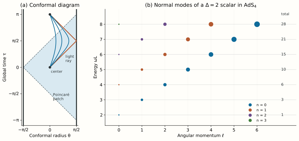
The diagram of Figure 1(a) shows the causal structure on a slice through the center, where the two ends $\theta =\pm \pi /2$ are opposite points of the boundary sphere. A radial light ray obeys $d\tau =\pm d\theta$ in these coordinates, so

$$\Delta \tau ={\int }_0^{\pi /2}d\theta =\frac{\pi }{2}$$

from the center to the boundary: light reaches infinity in finite global time. But the spatial proper distance to the boundary, $L\int d\rho$, is infinite. The travel time is finite because the lapse $\cosh \rho$ grows with $\rho$, so that light covers coordinate distance ever faster. Timelike geodesics behave very differently. For a massive particle moving radially through the center, the conserved energy and the normalization of the velocity give (Problem 7)

$$\sin \theta (\tau )=k\sin \tau ,0<k<1,$$

or equivalently $\tanh \rho =k\sin \tau$. Every such geodesic passes the center at $\tau =0$, comes to rest at its maximal radius at $\tau =\pi /2$, and returns to the center at $\tau =\pi$, independently of $k$.

Physical picture: AdS is a box with a harmonic trap inside. A massive particle is pulled back toward the center with a period $2\pi$ in global time, whatever its energy, as in a harmonic potential. A light ray escapes to the boundary in time $\pi /2$ and, if it is reflected there, returns at time $\pi$. The geometry therefore behaves as a finite box even though its spatial volume is infinite, and the evolution inside is determined only after a boundary condition is specified at $\theta =\pi /2$. This is the observation of Avis, Isham and Storey. The discrete spectrum of §7, with its uniform spacing, is the quantum version of the common period.

Checkpoint 1. Why does the finite travel time of light to the boundary require a boundary condition, while the infinite spatial distance does not prevent signals from arriving there?

Answer. The travel time is the relevant quantity for the initial-value problem: a signal can leave the interior, reach the boundary and return in a finite time, so data on a Cauchy slice do not determine the future without a rule at the boundary. The spatial distance measures a different integral, with the lapse removed.

4. The Poincaré patch

A second chart covers half of the hyperboloid. Set

$$X_0+X_d=\frac{L^2}{z},X_0-X_d=z+\frac{{\mathbf{x}}^2-t^2}{z},X_{d+1}=\frac{Lt}{z},X_i=\frac{L{x}_i}{z}(i=1,\dots ,d-1),$$

with $z>0$. The constraint is satisfied, and the induced metric is (Problem 8)

$$d{s}^2=\frac{L^2}{z^2}\left(d{z}^2-d{t}^2+d{\mathbf{x}}^2\right),z>0.$$

The boundary is at $z=0$, where the rescaled metric is Minkowski space, and the surface $z\to \infty$ is the Poincaré horizon, a null surface through which geodesics pass in finite affine parameter. The chart covers the region $X_0+X_d>0$. In the diagram of Figure 1(a) this is the shaded wedge bounded by the null lines $\tau =\pm (\theta +\pi /2)$; for AdS${}_2$ the explicit map is $t=L\sin \tau /(\cos \tau +\sin \theta )$ and $z=L\cos \theta /(\cos \tau +\sin \theta )$. At the boundary the condition $X_0+X_d>0$ reads $\cos \tau +\cos \psi >0$, where $\psi$ is the polar angle on $S^{d-1}$ measured from the image of the origin. The boundary Minkowski space is thus conformally mapped onto the diamond $|\tau |+\psi <\pi$ of the boundary cylinder, with spatial infinity at $\psi =\pi$ and $\tau =0$; along the edge $\theta =\pi /2$ of Figure 1(a), where $\psi =0$, the range is $-\pi <\tau <\pi$. This is the familiar embedding of Minkowski space into the Einstein static universe.

The transformation $(z,x^{\mu })\mapsto (\lambda z,\lambda x^{\mu })$ is an isometry. At fixed time the radial proper distance between $z_1$ and $z_2$ is $L\log (z_2/z_1)$, so equal multiplicative changes of $z$ are equal distances, and a change of boundary scale corresponds to a displacement in $z$. The Euclidean continuation $t=-i{t}_E$ gives the upper half-space $\frac{L^2}{z^2}(d{z}^2+d{\mathbf{x}}^2)$, which is hyperbolic space $H^{d+1}$, with conformal boundary ${\mathbb{R}}^d\cup \{\infty \}=S^d$. This is the geometry of the calculation in Lecture 15, and its boundary is the Euclidean space of radial quantization with its point at infinity.

The isometries of the Poincaré patch can now be matched with the conformal generators one by one. Translations and rotations of $x^{\mu }$ are manifest. The dilatation is generated by

$${\xi }_D=z{\partial }_z+x^{\mu }{\partial }_{\mu },$$

and in Euclidean signature the special conformal transformations by

$${\xi }_b=2(b\cdot x)\left(x^{\mu }{\partial }_{\mu }+z{\partial }_z\right)-\left(x^2+z^2\right)b^{\mu }{\partial }_{\mu }.$$

Both satisfy Killing’s equation for the Poincaré metric, and at $z=0$ they reduce to the conformal Killing vectors $\lambda x^{\mu }$ and $2(b\cdot x)x^{\mu }-x^2{b}^{\mu }$ of Lecture 12 (Problem 9). [Exact calculation.] The isometry group of the bulk acts on the conformal boundary as the conformal group of the boundary. This is the kinematical content of the correspondence, and it holds before any dynamics is specified. The Killing vector that Lecture 22 attaches to a boundary ball is one combination of these.

Checkpoint 2. Is the Poincaré horizon a singularity?

Answer. It is a coordinate boundary of the chart. The curvature is constant there, and the global coordinates continue smoothly across it into the rest of the hyperboloid.

5. A scalar field near the boundary

Consider a probe scalar satisfying $(\square -m^2)\varphi =0$ on a fixed AdS background. In the Poincaré chart,

$$z^2{\partial }_z^2\varphi -(d-1)z{\partial }_z\varphi +z^2{\square }_x\varphi -m^2{L}^2\varphi =0,$$

where ${\square }_x$ is the flat wave operator along the boundary. Near $z=0$ the boundary-derivative term is subleading for smooth data of fixed momentum, and the power $\varphi \sim z^{\alpha }$ solves the equation when

$$\alpha (\alpha -d)=m^2{L}^2.$$

Writing $\nu =\sqrt{d^2/4+m^2{L}^2}$, the two roots are

$${\alpha }_{\pm }=\frac{d}{2}\pm \nu ,\Delta \equiv {\alpha }_{+},m^2{L}^2=\Delta (\Delta -d).$$

For generic $\nu$ every solution therefore behaves as

$$\varphi (z,x)=z^{d-\Delta }\left[J(x)+\dots \right]+z^{\Delta }\left[A(x)+\dots \right].$$

Lecture 15 identifies $J$ with a source and relates $A$ to the expectation value of the dual operator. When the two exponents differ by an even integer, logarithms appear, and the two displayed terms are not a complete expansion.

Reality of $\nu$ requires

$$m^2{L}^2\ge -\frac{d^2}{4},$$

the Breitenlohner–Freedman bound. A negative mass squared is compatible with stability in AdS, because the box of §3 raises the energy of every mode. Section 7 shows that the bound is precisely the condition for the frequencies of the field to be real.

6. Which falloff can fluctuate

The Klein–Gordon inner product on a surface of constant $t$ contains the radial measure $\sqrt{-g}{g}^{tt}\propto z^{1-d}$. For a mode with falloff $z^{\alpha }$ its near-boundary contribution behaves as

$${\int }_{0}dz{z}^{2\alpha +1-d},$$

which converges when $\alpha >(d-2)/2$. The fast falloff ${\alpha }_{+}=\Delta$ always satisfies this condition. The slow falloff satisfies it when $0<\nu <1$. In that window both falloffs are normalizable, either may be held fixed, and the alternate quantization of Breitenlohner and Freedman gives an operator of dimension ${\Delta }_{-}=d/2-\nu$. Note that the threshold $\alpha >(d-2)/2$ is exactly the scalar unitarity bound of Lecture 12. The bulk norm and the boundary representation theory locate the same number, which is the first nontrivial check between the two descriptions.

For example, take AdS${}_4$ with $m^2{L}^2=-2$. Then $\nu =1/2$, the two falloffs are $z$ and $z^2$, and both $\Delta =2$ and $\Delta =1$ are admissible with the corresponding boundary conditions. This is the conformally coupled scalar of Lecture 15. At $\nu =0$ the two roots coincide and logarithms require separate treatment; at $\nu =1$ the slow falloff sits exactly at the unitarity bound.

7. The global spectrum

In global coordinates the field can be quantized directly. Separate variables as $\varphi =e^{-i\omega \tau }{Y}_{\ell }(\Omega )f(\theta )$, where the spherical harmonic satisfies ${\nabla }_{S^{d-1}}^2{Y}_{\ell }=-\ell (\ell +d-2)Y_{\ell }$, and $\omega$ is measured in units of $1/L$. In the coordinates of §3 the Klein–Gordon equation becomes

$$\frac{{\cos }^{d-1}\theta }{{\sin }^{d-1}\theta }\frac{d}{d\theta }\left({\tan }^{d-1}\theta \frac{df}{d\theta }\right)+{\omega }^{2}f-\frac{\ell (\ell +d-2)}{{\sin }^2\theta }f-\frac{m^2{L}^2}{{\cos }^2\theta }f=0.$$

Near the center regularity selects $f\sim {\sin }^{\ell }\theta$, and near the boundary the two solutions behave as ${\cos }^{\Delta }\theta$ and ${\cos }^{d-\Delta }\theta$, which are the two falloffs of §5 in these coordinates. The substitution $f={\cos }^{\Delta }\theta {\sin }^{\ell }\theta F(y)$ with $y={\sin }^2\theta$ turns the equation into the hypergeometric equation, and the solution regular at the center is

$$F(y)={}_2{F}_1(a,b;c;y),a=\frac{\Delta +\ell -\omega }{2},b=\frac{\Delta +\ell +\omega }{2},c=\ell +\frac{d}{2}.$$

At the boundary, $y\to 1$, the connection formula of the hypergeometric function gives

$${}_2{F}_1(a,b;c;y)=\frac{\Gamma (c)\Gamma (-\nu )}{\Gamma (c-a)\Gamma (c-b)}\left[1+\dots \right]+\frac{\Gamma (c)\Gamma (\nu )}{\Gamma (a)\Gamma (b)}(1-y{)}^{-\nu }\left[1+\dots \right],$$

because $c-a-b=-\nu$. The second term multiplies ${\cos }^{\Delta }\theta$ by ${\cos }^{-2\nu }\theta$, which is the slow falloff ${\cos }^{d-\Delta }\theta$. Standard quantization forbids it, so $1/\Gamma (a)$ must vanish, $a=-n$ with $n=0,1,2,\dots$, and

$$\boxed{{\omega }_{n\ell }=\Delta +2n+\ell ,n,\ell =0,1,2,\dots }$$

[Exact calculation.] The negative frequencies $b=-n$ give the complex-conjugate modes. For a generic $\omega$ the coefficient of the slow falloff is nonzero, so only this discrete set satisfies both conditions.

The spectrum reproduces the conformal family of Lecture 12. The lowest mode, $n=\ell =0$, is $e^{-i\Delta \tau }{\cos }^{\Delta }\theta$ and has energy $\Delta$: it is the primary state $|\mathcal{O}⟩$ on a boundary cylinder of radius $L$ (Problem 6). The level $\omega =\Delta +k$ collects all pairs with $2n+\ell =k$, and its total degeneracy is

$$\sum _{\begin{array}{c}n,\ell \ge 0\\ 2n+\ell =k\end{array}}\dim {\mathcal{H}}_{\ell }(S^{d-1})=\left(\genfrac{}{}{0ex}{}{k+d-1}{d-1}\right),$$

where ${\mathcal{H}}_{\ell }(S^{d-1})$ is the space of spherical harmonics of degree $\ell$. The right side is the number of independent descendants $P_{{\mu }_1}\cdots P_{{\mu }_k}|\mathcal{O}⟩$ at level $k$, since for generic $\Delta$ there are no null states (Problem 10). In $d=3$ the degeneracies are $1,3,6,10,\dots$, as Figure 1(b) shows. The single-particle Hilbert space of a free scalar in AdS is therefore exactly one conformal family, with primary dimension $\Delta$. [Exact calculation.] The identity $m^2{L}^2=\Delta (\Delta -d)$, which §5 obtained from the boundary behavior, is here the statement that the conformal Casimir of the family equals the bulk mass.

Two consequences follow at once. First, the frequencies are real exactly when $\Delta$ is real, that is, when the Breitenlohner–Freedman bound of §5 holds. Below it $\Delta$ is complex and the modes grow exponentially in global time, so the bound is the condition of linear stability. Second, a free field has multi-particle states with energies that add. The two-particle states organize into conformal families whose primaries have $\omega =2\Delta +2n+\ell$, with even $\ell$ for identical particles, which are the dimensions of the double-trace families of a generalized free field in Lecture 12. Interactions in the bulk shift these energies, and the shifts are the anomalous dimensions that Lecture 14 counts in powers of $1/N$.

8. What the geometry supplies

At this point the geometry has supplied three things without any assumption about a dual theory: a conformal boundary on which the isometries act as the conformal group, a causal structure that requires boundary conditions, and a free-field spectrum that is organized into conformal families. The correspondence adds two further statements. The boundary conditions are identified with sources for operators of a CFT, which is the prescription of Lecture 15. And the bulk is described by a small number of weakly coupled fields, which requires the large-$N$ structure of Lecture 14. The free field of this lecture is the leading term of that description, and it reproduces a generalized free field on the boundary.

9. What to take away

• Exact: AdS${}_{d+1}$ has isometry group $SO(d,2)$ and a conformal boundary $\mathbb{R}\times S^{d-1}$; global time translation acts on the boundary as the dilatation operator of Lecture 12.
• Exact: light reaches the boundary in global time $\pi /2$, while timelike geodesics through the center return to it after a global time $\pi$ and oscillate with period $2\pi$; the evolution requires boundary conditions.
• Exact: in the Poincaré patch the Killing vectors reduce at $z=0$ to the conformal Killing vectors of Minkowski space.
• Exact: a scalar of mass $m^2{L}^2=\Delta (\Delta -d)$ has falloffs $z^{d-\Delta }$ and $z^{\Delta }$; both are normalizable for $0<\nu <1$, the window of the alternate quantization.
• Exact: the normalizable global modes have $\omega =\Delta +2n+\ell$, and their degeneracies reproduce one conformal family; the Breitenlohner–Freedman bound is the reality of these frequencies.

10. Looking ahead

Lecture 14 explains why a quantum theory with many degrees of freedom can be described, at leading order, by a few free fields of this kind, and what controls the corrections. Lecture 15 then turns the boundary behavior of §5 into the dictionary between sources, expectation values and correlators, and Lecture 16 uses the Poincaré geometry of §4 to compute an entropy from a geodesic length.

11. Problem set

Classroom core

1. The curvature scale. Insert $R_{\mu \nu }=-d{g}_{\mu \nu }/L^2$ into Einstein’s vacuum equation with a cosmological constant and find $\Lambda$.

2. The conformal boundary. Derive the metric of §3 from $\tan \theta =\sinh \rho$, and compute the global time for a radial light ray to travel from the center to the boundary and back.

3. A negative mass squared. For $d=3$ and $m^2{L}^2=-2$, compare with the stability threshold, and find both admissible dimensions.

4. Normalizability. Test the falloffs $z$ and $z^2$ in AdS${}_4$ against the Klein–Gordon norm of §6.

5. Quantization. Show that normalizability at the boundary gives $\omega =\Delta +2n+\ell$. For $d=3$ and $\Delta =2$, list the energies up to $\omega =5$ with their degeneracies and compare them with the descendants of a scalar primary in Lecture 12.

6. The primary mode. Verify that $e^{-i\Delta \tau }{\cos }^{\Delta }\theta$ solves the Klein–Gordon equation with $m^2{L}^2=\Delta (\Delta -d)$.

Self-study consolidation

7. Timelike geodesics. Use the conserved energy $E=\dot{\tau }/{\cos }^2\theta$ and the normalization of the velocity to show that radial timelike geodesics satisfy $\sin \theta =k\sin \tau$ with $E^2=1/(1-k^2)$, in units $L=1$.

8. The Poincaré embedding. Verify that the embedding of §4 satisfies the constraint and induces the Poincaré metric, and show that it covers the region $X_0+X_d>0$.

9. Isometries and conformal maps. Verify that ${\xi }_D$ and ${\xi }_b$ are Killing vectors of Euclidean Poincaré AdS and that they reduce at $z=0$ to the conformal Killing vectors of Lecture 12.

10. The degeneracy identity. Show that ${\sum }_{2n+\ell =k}\dim {\mathcal{H}}_{\ell }(S^{d-1})=\left(\genfrac{}{}{0ex}{}{k+d-1}{d-1}\right)$. Hint: homogeneous polynomials of degree $k$ in $d$ variables decompose as ${\mathcal{P}}_k={\mathcal{H}}_k\oplus r^2{\mathcal{P}}_{k-2}$.

11. Scale covariance of the source. A source for an operator of dimension $\Delta$ couples as $\int d^{d}xJ\mathcal{O}$. Find the dimension of $J$ and compare with the coefficient of $z^{d-\Delta }$.

12. Coordinate time and proper distance. Explain why a null signal can reach the boundary in finite $\tau$ although a spatial radial path has infinite length.

Research extension

13. Boundary conditions as self-adjoint extensions. For $0<\nu <1$, show that mixed boundary conditions relating the coefficients of the two falloffs form a one-parameter family of well-defined evolutions, determine for which sign of the mixing parameter the energy is positive, and find the spectrum for the alternate quantization. Known: the analysis of Ishibashi and Wald, and the double-trace interpretation of Lecture 15. Completion: the frequencies for the two pure boundary conditions and the equation that determines them for a mixed one.

14. Below the bound. For $m^2{L}^2<-d^2/4$, write $\nu =i\mu$. Show that the formal solutions with $\Delta =d/2+i\mu$ have complex frequencies, and that no self-adjoint boundary condition makes the energy bounded below. Known: the Breitenlohner–Freedman analysis and the self-adjoint extensions of Problem 13. Completion: the complex frequencies, the boundary condition to which they correspond, and the argument that every self-adjoint extension is unbounded below.

15. Two-particle energies. For two free scalars of dimension $\Delta$, construct the two-particle state of lowest energy and identify it with $[\mathcal{OO}{]}_{0,0}$. Add a contact interaction $\frac{\lambda }{4!}{\varphi }^4$ and compute the first-order shift of its energy. Known: this shift is the anomalous dimension of the double-trace operator, of order $1/N^2$ in the normalization of Lecture 14. Completion: the shift as an overlap integral of the primary mode, evaluated for one value of $\Delta$ and $d$.

12. Answer checkpoints

1. $R_{\mu \nu }-\frac{1}{2}R{g}_{\mu \nu }+\Lambda g_{\mu \nu }=\left[-\frac{d}{L^2}+\frac{d(d+1)}{2L^2}+\Lambda \right]g_{\mu \nu }=0$ gives $\Lambda =-d(d-1)/(2L^2)$.

2. With $\cosh \rho =1/\cos \theta$ and $d\rho =d\theta /\cos \theta$, each term of the global metric acquires the factor $1/{\cos }^2\theta$ and ${\sinh }^2\rho ={\tan }^2\theta$. A radial light ray has $d\tau =d\theta$, so it reaches $\theta =\pi /2$ at $\tau =\pi /2$ and, after reflection, the center at $\tau =\pi$.

3. The threshold is $-9/4$, so $-2$ lies above it; $\nu =1/2$ and the dimensions are $2$ and $1$.

4. The norm integrands behave as $z^{2\alpha +1-d}$, that is $z^0$ for $\alpha =1$ and $z^2$ for $\alpha =2$; both are integrable at $z=0$.

5. The coefficient of the slow falloff is proportional to $1/\Gamma (a)$, which vanishes only at $a=-n$, giving $\omega =\Delta +\ell +2n$. For $d=3$ and $\Delta =2$: $\omega =2$ with degeneracy 1; $\omega =3$ with $\ell =1$, degeneracy 3; $\omega =4$ with $(n,\ell )=(1,0),(0,2)$, degeneracy $1+5=6$; $\omega =5$ with $(1,1),(0,3)$, degeneracy $3+7=10$. These are the numbers of descendants $1,3,6,10$ at levels $0,1,2,3$.

6. For $\ell =0$ and $f={\cos }^{\Delta }\theta$, a direct computation gives $\frac{{\cos }^{d-1}\theta }{{\sin }^{d-1}\theta }{\partial }_{\theta }\left({\tan }^{d-1}\theta {\partial }_{\theta }{\cos }^{\Delta }\theta \right)=-{\Delta }^2{\cos }^{\Delta }\theta +\Delta (\Delta -d){\cos }^{\Delta -2}\theta$. The first term cancels ${\omega }^{2}f$ with $\omega =\Delta$, and the second cancels the mass term $m^2{L}^2{\cos }^{\Delta -2}\theta$.

7. The normalization $\frac{1}{{\cos }^2\theta }(-{\dot{\tau }}^2+{\dot{\theta }}^2)=-1$ gives $d\theta /d\tau =\sqrt{E^2{\cos }^2\theta -1}/(E\cos \theta )$. Substituting $\sin \theta =k\sin \tau$ makes both sides equal to $k\cos \tau /\cos \theta$ when $E^2=1/(1-k^2)$.

8. The constraint becomes $-(X_0+X_d)(X_0-X_d)-X_{d+1}^2+{\sum }_i{X}_i^2=-L^2$ identically. The induced metric follows by differentiating, and $z>0$ is equivalent to $X_0+X_d>0$.

9. The Lie derivative of $L^2{z}^{-2}(d{z}^2+d{\mathbf{x}}^2)$ along ${\xi }_D$ vanishes because the metric is scale invariant. For ${\xi }_b$ the $z$-dependence of $x^2+z^2$ and the term $2(b\cdot x)z{\partial }_z$ cancel the rescaling of the conformal factor. At $z=0$ the vectors become $x^{\mu }{\partial }_{\mu }$ and $2(b\cdot x)x^{\mu }{\partial }_{\mu }-x^2{b}^{\mu }{\partial }_{\mu }$.

10. The decomposition gives $\dim {\mathcal{P}}_k=\dim {\mathcal{H}}_k+\dim {\mathcal{P}}_{k-2}$. Iterating, $\dim {\mathcal{P}}_k={\sum }_n\dim {\mathcal{H}}_{k-2n}$, and $\dim {\mathcal{P}}_k=\left(\genfrac{}{}{0ex}{}{k+d-1}{d-1}\right)$.

11. $[J]=d-\Delta$, which is also the power of $z$ multiplying $J$, so that $z^{d-\Delta }J$ is scale invariant under $(z,x)\mapsto (\lambda z,\lambda x)$.

12. The lapse grows as $\cosh \rho$, so the coordinate speed of light $d\rho /d\tau =\cosh \rho$ grows toward the boundary. The time integral $\int d\rho /\cosh \rho$ converges while the length $\int d\rho$ diverges.

13. Guide. Write the radial operator as a Sturm–Liouville operator and compute its deficiency indices; for $0<\nu <1$ both falloffs are square integrable and a one-parameter family of self-adjoint extensions exists. The alternate quantization gives $\omega ={\Delta }_{-}+2n+\ell$, and a mixed condition gives a transcendental equation for the frequencies. For one sign of the mixing parameter, which corresponds to a negative double-trace coupling in Lecture 15, a mode with imaginary frequency appears.

14. Guide. With $\Delta =d/2+i\mu$ the formal frequencies $\omega =d/2+i\mu +2n+\ell$ grow as $e^{\mu \tau }$, but they correspond to a complex boundary condition, which is not self-adjoint. For every self-adjoint extension the radial operator is unbounded below, so there are growing modes with arbitrarily large rates; this is why no boundary condition restores stability.

15. Guide. The lowest two-particle state is $(a_{00}^{†}{)}^2|0⟩/\sqrt{2}$, with energy $2\Delta$. First-order perturbation theory gives a shift proportional to $\lambda \int d^{d}x\sqrt{-g}|f_{00}{|}^4$ with the normalized primary mode, which is the anomalous dimension of $[\mathcal{OO}{]}_{0,0}$.

Wiki connections. holographic dictionary