Lecture 15 — A complete scalar source and response calculation

Maldacena’s correspondence became a tool for calculation when Gubser, Klebanov and Polyakov, and independently Witten, stated how a source in the boundary theory enters the bulk. This lecture carries out their prescription completely for a free scalar of arbitrary mass in Euclidean Poincaré AdS. We solve the boundary-value problem, evaluate the on-shell action at a cutoff, remove its divergence with a local counterterm, and differentiate the result. The outcome is the two-point function of a scalar primary of dimension $\Delta$, including the factor $2\Delta -d$ in its normalization, which was settled only after Freedman, Mathur, Matusis and Rastelli examined how the boundary limit must be taken. The conformally coupled scalar in AdS${}_4$ is the case in which every coefficient can be checked by hand.

How to use this lecture

Classroom core, two meetings of two hours. The first meeting states the prescription and its origin (§1, 15 minutes), sets up and solves the boundary-value problem (§§2–3, 40 minutes), and carries the conformally coupled example through to its renormalized action and two-point function (§4, 50 minutes), leaving 15 minutes for Checkpoints 1 and 2. The second meeting derives the general counterterm and the factor $2\Delta -d$ (§5, 35 minutes) and constructs the bulk-to-boundary propagator and the position-space correlator (§6, 35 minutes). It closes with the alternate quantization and the large-$N$ reading of the result (§8.1 and §9, 30 minutes), leaving 20 minutes for Problems 1–4; Problems 5 and 6 complete the core assignment. These allocations are proposals and have not been tested in class.

Self-study. Section 7 compares three ways of taking the boundary limit and explains the historical normalization issue. Section 8.2 derives the same factor from the extrapolate form of the dictionary used in Lecture 18, and §10 treats masses that require a second counterterm. Problems 7–12 consolidate these steps.

Research extension. Section 11 outlines Lorentzian response functions, three-point functions from a cubic bulk coupling, and double-trace flows between the two quantizations, with Problems 13–15.

Prerequisites. Lecture 12 for the two- and three-point functions of scalar primaries and the unitarity bound; Lecture 13 for Poincaré AdS, the indicial equation, normalizability and the Breitenlohner–Freedman bound; Lecture 14 for large-$N$ counting. We also use Fourier transforms, integration by parts, functional derivatives, and the modified Bessel functions $I_{\nu }$ and $K_{\nu }$, whose needed properties are recalled where they enter.

What this lecture establishes. Sections 2–8 and 10 are exact calculations for a free scalar on a fixed Euclidean AdS background. The identification of the renormalized on-shell action with the generating functional of a CFT is the holographic input stated in §1. The large-$N$ reading of §9 is controlled by the bulk loop expansion, whose terms we do not compute.

0. Reading

Primary.

• J. Maldacena, The Large N Limit of Superconformal Field Theories and Supergravity (1997).
• S. S. Gubser, I. R. Klebanov, A. M. Polyakov, Gauge Theory Correlators from Non-Critical String Theory (1998).
• E. Witten, Anti De Sitter Space and Holography (1998).

Secondary.

• D. Z. Freedman, S. D. Mathur, A. Matusis, L. Rastelli, Correlation functions in the CFT(d)/AdS(d+1) correspondence (1998): the normalization discussed in §7 and the three-point functions of §11.2.
• I. R. Klebanov, E. Witten, AdS/CFT Correspondence and Symmetry Breaking (1999): the alternate quantization of §8.1.
• S. de Haro, K. Skenderis, S. N. Solodukhin, Holographic Reconstruction of Spacetime and Renormalization in the AdS/CFT Correspondence (2000), and K. Skenderis, Lecture Notes on Holographic Renormalization (2002): the counterterms of §§5 and 10.
• J. Penedones, TASI lectures on AdS/CFT (2016), and D. Harlow, TASI Lectures on the Emergence of the Bulk in AdS/CFT (2018), Sections 2–3: gentler accounts of the same material.

Optional research reading.

• T. Banks, M. R. Douglas, G. T. Horowitz, E. Martinec, AdS Dynamics from Conformal Field Theory (1998), and D. Harlow, D. Stanford, Operator Dictionaries and Wave Functions in AdS/CFT and dS/CFT (2011): the extrapolate dictionary of §8.2.
• D. T. Son, A. O. Starinets, Minkowski-space correlators in AdS/CFT correspondence: recipe and applications (2002), and K. Skenderis, B. C. van Rees, Real-time gauge/gravity duality (2008): §11.1.
• E. Witten, Multi-Trace Operators, Boundary Conditions, And AdS/CFT Correspondence (2001); I. R. Klebanov, A. M. Polyakov, AdS Dual of the Critical O(N) Vector Model (2002); T. Hartman, L. Rastelli, Double-Trace Deformations, Mixed Boundary Conditions and Functional Determinants in AdS/CFT (2006): §11.3.
• L. Susskind, E. Witten, The Holographic Bound in Anti-de Sitter Space (1998): the relation between depth and resolution in §6.

1. From a duality to a rule for correlators

In November 1997 Maldacena compared two descriptions of the low-energy physics of $N$ coincident D3-branes and argued that $\mathcal{N}=4$ super-Yang–Mills theory with gauge group $SU(N)$ is equivalent to type IIB string theory on AdS${}_5\times S^5$. His argument matched the symmetries on the two sides and identified the regime in which each is tractable; Lecture 14 examined the large-$N$ counting behind it. What it did not yet provide was a rule for computing a correlation function of the gauge theory from the bulk. That rule appeared three months later, in two papers submitted within a week of each other. Gubser and Klebanov had computed, partly with Tseytlin, how a stack of D3-branes absorbs low-energy gravitons and dilatons, and had found that the absorption cross-section is controlled by the two-point function of the gauge-theory operator to which the incoming field couples. Together with Polyakov, whose work on confining strings had suggested a five-dimensional description of four-dimensional gauge theory, they proposed that the dependence of the supergravity action on the boundary values of its fields is the generating functional of gauge-theory correlators. Witten reached the same prescription by emphasizing the conformal boundary of AdS and the holographic ideas of ‘t Hooft and Susskind, and he showed that the masses of bulk fields determine the dimensions of the dual operators.

For a scalar primary $\mathcal{O}$ of dimension $\Delta$ the prescription pairs $\mathcal{O}$ with a bulk field $\varphi$ of mass $m^2{L}^2=\Delta (\Delta -d)$, as in Lecture 13, and states

$$Z_{\mathrm{CFT}}[J]=⟨\exp \int d^{d}xJ(\mathbf{x})\mathcal{O}(\mathbf{x})⟩=Z_{\mathrm{bulk}}\left[\varphi \to z^{d-\Delta }J\right],$$

where the right side is the bulk partition function computed with the condition that the leading behavior of $\varphi$ near the boundary $z=0$ be $z^{d-\Delta }J(\mathbf{x})$. When the bulk is classical, the path integral is dominated by the solution ${\varphi }_J$ with this behavior, and

$$W[J]\equiv \log Z_{\mathrm{CFT}}[J]=-I_{\mathrm{ren}}[{\varphi }_J]+\dots ,$$

where $I_{\mathrm{ren}}$ is the renormalized Euclidean action constructed in §§4–5 and the dots denote bulk loop corrections. These are suppressed by the inverse of the overall normalization of the bulk action, that is, by $G_N/L^{d-1}\sim N^{-2}$. Connected correlators follow by differentiation,

$$⟨\mathcal{O}({\mathbf{x}}_1)\cdots \mathcal{O}({\mathbf{x}}_n){⟩}_c={\frac{{\delta }^{n}W}{\delta J({\mathbf{x}}_1)\cdots \delta J({\mathbf{x}}_n)}|}_{J=0}.$$

[Stated only — refs: Gubser, Klebanov, Polyakov; Witten.] This is the holographic input of the lecture, and the course takes it as given. Its content lies in the consistency checks it passes, and the calculation below is the first of them: the right side must reproduce the two-point function $C_{\mathcal{O}}/|\mathbf{x}-\mathbf{y}{|}^{2\Delta }$, with $C_{\mathcal{O}}>0$, that conformal symmetry and reflection positivity require in Lecture 12.

Physical picture: a boundary condition changes the theory. Lecture 13 showed that a light ray reaches the conformal boundary of AdS in finite global time, so bulk evolution is determined only after something is specified there. The two falloffs $z^{d-\Delta }$ and $z^{\Delta }$ play different roles in that specification. In standard quantization the coefficient of $z^{\Delta }$ fluctuates and describes states, while the coefficient of $z^{d-\Delta }$ is held fixed. Fixing it at a nonzero value changes the theory itself, and the prescription identifies this change with the deformation of the CFT action by $\int J\mathcal{O}$. A source and an expectation value are therefore the two integration constants of a single radial equation, and the dictionary is the map between them that solving the bulk equation computes. The picture is exact for the free field of this lecture; its reading as a statement about a CFT is the input stated above.

2. The boundary-value problem

Consider Euclidean AdS${}_{d+1}$ in Poincaré coordinates,

$$d{s}^2=\frac{L^2}{z^2}\left(d{z}^2+d{\mathbf{x}}^2\right),z>0,\mathbf{x}\in {\mathbb{R}}^d,$$

and a free scalar with action

$$I[\varphi ]=\frac{\mathcal{N}}{2}{\int }_{z\ge ϵ}{d}^{d+1}x\sqrt{g}\left(g^{ab}{\partial }_a\varphi {\partial }_b\varphi +m^2{\varphi }^2\right),m^2{L}^2=\Delta (\Delta -d),$$

where $ϵ$ is a radial cutoff removed at the end and $\mathcal{N}>0$ is the overall normalization of the action. We write

$$\nu =\Delta -\frac{d}{2}>0,$$

so that $\Delta$ is the larger root ${\Delta }_{+}$ of Lecture 13, and we take $\nu$ non-integer throughout; §5 assumes $0<\nu <1$, and §10 removes that restriction. For a scalar that descends from a gravitational action $\mathcal{N}$ is proportional to $1/G_N$, and every correlator below is proportional to $\mathcal{N}$, which is why we keep it explicit. The sign conventions are those of the course conventions sheet: $Z[J]=⟨e^{\int J\mathcal{O}}⟩$, $W=\log Z\simeq -I_{\mathrm{ren}}$, and the unit normal to the cutoff surface points out of the region $z\ge ϵ$, toward decreasing $z$, so that $n^z=-z/L$.

Varying the action and integrating by parts,

$$\delta I=\mathcal{N}{\int }_{z\ge ϵ}{d}^{d+1}x\sqrt{g}\delta \varphi \left(-\square +m^2\right)\varphi +\mathcal{N}{\int }_{z=ϵ}{d}^{d}x\sqrt{\gamma }\delta \varphi n^a{\partial }_a\varphi ,$$

where $\gamma$ is the induced metric on the cutoff surface, with $\sqrt{\gamma }=(L/ϵ{)}^d$. The bulk term gives the Klein–Gordon equation $(\square -m^2)\varphi =0$. The boundary term will matter twice: evaluated on a solution the whole action reduces to it, and requiring the renormalized variational problem to be well posed will fix the counterterms.

Fourier transforming along the boundary, $\varphi (z,\mathbf{x})={\int }_{\mathbf{k}}{e}^{i\mathbf{k}\cdot \mathbf{x}}\varphi (z,\mathbf{k})$ with ${\int }_{\mathbf{k}}\equiv \int d^{d}k/(2\pi {)}^d$ and $k=|\mathbf{k}|$, the Klein–Gordon equation becomes the radial equation

$$z^2{\partial }_z^2\varphi -(d-1)z{\partial }_z\varphi -\left(k^2{z}^2+m^2{L}^2\right)\varphi =0.$$

Near $z=0$ the term $k^2{z}^2$ is negligible, and $z^{\alpha }$ solves the equation when $\alpha (\alpha -d)=m^2{L}^2$. This is the indicial equation of Lecture 13, with roots $d-\Delta$ and $\Delta$. Every solution therefore behaves as

$$\varphi (z,\mathbf{k})=z^{d-\Delta }\left[J(\mathbf{k})+O(z^2)\right]+z^{\Delta }\left[A(\mathbf{k})+O(z^2)\right],$$

and standard quantization declares $J$ the source. The corrections of order $z^2$ are fixed by $J$ and $A$ through the radial equation (Problem 2). Once $J$ is given, the coefficient $A$ is determined by the behavior of the solution deep in the bulk.

3. Regularity in the interior fixes the response

The substitution $\varphi =z^{d/2}f(kz)$ turns the radial equation into

$$u^2{f}^{\prime \prime }(u)+u{f}^{\prime }(u)-\left(u^2+{\nu }^2\right)f(u)=0,u=kz,$$

the modified Bessel equation of order $\nu$, because $d^2/4+m^2{L}^2={\nu }^2$ (Problem 1). Its solutions are $I_{\nu }(u)$, which grows as $e^u/\sqrt{2\pi u}$, and $K_{\nu }(u)$, which decays as $\sqrt{\pi /2u}{e}^{-u}$. As $z\to \infty$ at fixed $\mathbf{x}$ one approaches the point at infinity of the boundary of hyperbolic space, and a solution that grows exponentially there has infinite action. Regularity, the Euclidean condition that selects the vacuum, therefore keeps $K_{\nu }$.

For non-integer $\nu$ the small-argument behavior of $K_{\nu }$ follows from $K_{\nu }=\frac{\pi }{2\sin \nu \pi }\left(I_{-\nu }-I_{\nu }\right)$, the power series of $I_{\pm \nu }$, and the reflection formula $\Gamma (\nu )\Gamma (1-\nu )=\pi /\sin \nu \pi$:

$$K_{\nu }(u)=\frac{\Gamma (\nu )}{2}{\left(\frac{u}{2}\right)}^{-\nu }\left[1+O(u^2)\right]+\frac{\Gamma (-\nu )}{2}{\left(\frac{u}{2}\right)}^{\nu }\left[1+O(u^2)\right].$$

Normalizing the leading term to $z^{d-\Delta }J$, we obtain the regular solution

$${\varphi }_J(z,\mathbf{k})=\frac{2}{\Gamma (\nu )}{\left(\frac{k}{2}\right)}^{\nu }{z}^{d/2}{K}_{\nu }(kz)J(\mathbf{k}),$$

whose response coefficient is

$$A(\mathbf{k})=b_{\nu }(k)J(\mathbf{k}),b_{\nu }(k)=\frac{\Gamma (-\nu )}{\Gamma (\nu )}{\left(\frac{k}{2}\right)}^{2\nu }.$$

The function $b_{\nu }$ is the central object of the lecture. Note that it is a non-integer power of $k^2$. A polynomial in $k^2$ would describe a response built from derivatives of delta functions, local on the boundary, whereas $k^{2\nu }$ is the Fourier transform of a power law at separated points, as §6 will show. The nonlocality of the boundary correlator is thus a direct consequence of the condition imposed in the far interior. For $0<\nu <1$ the factor $\Gamma (-\nu )$ is negative, so $b_{\nu }<0$ in that range. But the position-space correlator will turn out positive for every $\nu$.

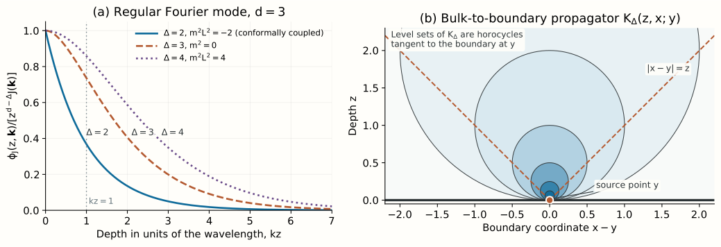
Physical picture: the response is fixed by the state in the interior. The boundary data fix only one of the two integration constants. The other is fixed by the condition at $z\to \infty$, which in Euclidean signature selects the vacuum. A different condition there, such as an incoming wave in Lorentzian signature (§11.1) or a regular horizon at finite depth in a thermal state (Lecture 23), produces a different response to the same source. Figure 1(a) shows the profile of the regular mode: it follows the source falloff near the boundary and decays once $kz$ exceeds a number of order one, so a source of wavenumber $k$ probes the bulk down to a depth of order $1/k$. The same principle returns throughout the course. The boundary correlator measures how the bulk state responds, and the interior condition is the bulk statement of which state that is.

4. The conformally coupled scalar in AdS${}_4$

Consider $d=3$ and $m^2{L}^2=-2$, so that $\nu =1/2$ and $\Delta =2$. This mass is special. A massless scalar with the conformal coupling $\frac{1}{6}R{\varphi }^2$ in four dimensions has effective mass squared $\frac{1}{6}R$, and in AdS${}_4$ the Ricci scalar is $R=-12/L^2$, so $m^2{L}^2=-2$ describes exactly the conformally coupled scalar. Since the metric is conformal to flat space, $g_{ab}=(L/z{)}^2{\delta }_{ab}$, a conformally coupled field is $\varphi =(z/L){\varphi }_{\mathrm{flat}}$ with ${\varphi }_{\mathrm{flat}}$ harmonic in flat space, which is why the radial equation reduces to an exponential. The same bulk field appears in a well-known holographic pair. Klebanov and Polyakov proposed that the singlet sector of the three-dimensional O(N) vector model is dual to Vasiliev’s higher-spin gravity in AdS${}_4$, whose scalar has precisely this mass. With one boundary condition it is dual to ${\varphi }^a{\varphi }^a$ of the free model, of dimension one, and with the other to the dimension-two operator of the large-$N$ critical model. These are the two roots $d-\Delta$ and $\Delta$ of §2, and §8.1 explains how both arise.

4.1 The solution

Since $K_{1/2}(u)=\sqrt{\pi /2u}{e}^{-u}$, the regular solution of §3 is

$${\varphi }_J(z,\mathbf{k})=z{e}^{-kz}J(\mathbf{k})=zJ(\mathbf{k})-k{z}^{2}J(\mathbf{k})+O(z^3).$$

Thus $A=-kJ$, in agreement with $b_{1/2}=\frac{\Gamma (-1/2)}{\Gamma (1/2)}\frac{k}{2}=-k$.

4.2 The on-shell action

On a solution the bulk term of the action vanishes after integration by parts, and the contribution from $z\to \infty$ vanishes because ${\varphi }_J$ decays there. What remains is

$$I_{\mathrm{os}}=\frac{\mathcal{N}}{2}{\int }_{z=ϵ}{d}^{3}x\sqrt{\gamma }\varphi n^a{\partial }_a\varphi =-\frac{\mathcal{N}{L}^2}{2}{\int }_{\mathbf{k}}{ϵ}^{-2}{\varphi }_J(ϵ,-\mathbf{k}){\partial }_z{\varphi }_J(ϵ,\mathbf{k}),$$

since $\sqrt{\gamma }=(L/ϵ{)}^3$ and $n^z=-ϵ/L$ at the cutoff. Substituting the solution,

$$I_{\mathrm{os}}=-\frac{\mathcal{N}{L}^2}{2}{\int }_{\mathbf{k}}J(-\mathbf{k})J(\mathbf{k})e^{-2kϵ}\left(\frac{1}{ϵ}-k\right)=-\frac{\mathcal{N}{L}^2}{2}{\int }_{\mathbf{k}}J(-\mathbf{k})J(\mathbf{k})\left(\frac{1}{ϵ}-3k+O(ϵ)\right).$$

Note that the exponential must be expanded together with the bracket; the bracket alone would give $-k$ where the finite coefficient is $-3k$. The divergent term multiplies $J(-\mathbf{k})J(\mathbf{k})$ with no dependence on $k$, so in position space it is ${ϵ}^{-1}\int d^{3}x{J}^2$, a local term.

4.3 The counterterm

Consider the boundary functional

$$I_{\mathrm{ct}}=\frac{\mathcal{N}}{2L}{\int }_{z=ϵ}{d}^{3}x\sqrt{\gamma }{\varphi }^2=\frac{\mathcal{N}{L}^2}{2}{\int }_{\mathbf{k}}J(-\mathbf{k})J(\mathbf{k})\frac{e^{-2kϵ}}{ϵ}=\frac{\mathcal{N}{L}^2}{2}{\int }_{\mathbf{k}}J(-\mathbf{k})J(\mathbf{k})\left(\frac{1}{ϵ}-2k+O(ϵ)\right).$$

It is built from the field on the cutoff surface and its induced metric, so it is a legitimate local counterterm of the regulated theory, and its coefficient is chosen to cancel the divergence of $I_{\mathrm{os}}$. But it also carries the finite term $-2k$, because the field at the cutoff already contains the response. Adding the two before taking the limit gives an expression that is exact at finite cutoff,

$$I_{\mathrm{os}}+I_{\mathrm{ct}}=\frac{\mathcal{N}{L}^2}{2}{\int }_{\mathbf{k}}k{e}^{-2kϵ}J(-\mathbf{k})J(\mathbf{k}),$$

and the renormalized action is

$$I_{\mathrm{ren}}=\underset{ϵ\to 0}{\lim }\left(I_{\mathrm{os}}+I_{\mathrm{ct}}\right)=\frac{\mathcal{N}{L}^2}{2}{\int }_{\mathbf{k}}kJ(-\mathbf{k})J(\mathbf{k}).$$

4.4 One- and two-point functions

With $W=-I_{\mathrm{ren}}$,

$$⟨\mathcal{O}(\mathbf{k}){⟩}_J=-\mathcal{N}{L}^{2}kJ(\mathbf{k})=\mathcal{N}{L}^{2}A(\mathbf{k}),G(\mathbf{k})=-\mathcal{N}{L}^{2}k,$$

where $⟨\mathcal{O}(\mathbf{x})\mathcal{O}(\mathbf{y})⟩={\int }_{\mathbf{k}}{e}^{i\mathbf{k}\cdot (\mathbf{x}-\mathbf{y})}G(\mathbf{k})$ up to contact terms. To return to position space we use

$$\int d^{d}x{e}^{-i\mathbf{k}\cdot \mathbf{x}}\frac{1}{|\mathbf{x}{|}^{2\Delta }}={\pi }^{d/2}{2}^{d-2\Delta }\frac{\Gamma (d/2-\Delta )}{\Gamma (\Delta )}{k}^{2\Delta -d},$$

which holds as a convergent integral for $(d-1)/4<\Delta <d/2$, and by analytic continuation in $\Delta$ elsewhere, away from $\Delta =d/2+n$, as a statement about separated points. At $d=3$ and $\Delta =2$ the coefficient is ${\pi }^{3/2}{2}^{-1}\Gamma (-1/2)=-{\pi }^2$, and therefore

$$⟨\mathcal{O}(\mathbf{x})\mathcal{O}(\mathbf{y})⟩=\frac{\mathcal{N}{L}^2}{{\pi }^2}\frac{1}{|\mathbf{x}-\mathbf{y}{|}^4},\mathbf{x}\ne \mathbf{y}.$$

This is the two-point function of a scalar primary of dimension two, with a positive coefficient, as Lecture 12 requires. The negative sign of $G(\mathbf{k})$ is consistent with it: the Fourier transform of $|\mathbf{x}{|}^{-4}$ in three dimensions is $-{\pi }^{2}k$ up to contact terms, and reflection positivity constrains the correlator at separated points.

Checkpoint 1. Which part of $I_{\mathrm{ren}}$ is fixed by the calculation, and which part depends on conventions?

Answer. The nonanalytic term $k$ is fixed. A finite local counterterm $\frac{a}{2}\int d^{3}x{J}^2$ would shift $G(\mathbf{k})$ by the constant $-a$, which is the contact term $-a{\delta }^{(3)}(\mathbf{x}-\mathbf{y})$ and leaves the separated-point correlator unchanged.

Checkpoint 2. Why does the finite coefficient of $I_{\mathrm{os}}$ alone, $-3k$, give the wrong correlator?

Answer. Subtractions must be local in the fields of the regulated theory. The counterterm is local in $\varphi (ϵ,\mathbf{x})$, and written in terms of $J$ it contains the finite term $-2k$. Discarding only the $1/ϵ$ term of $I_{\mathrm{os}}$ amounts to a subtraction that is nonlocal in $\varphi (ϵ,\mathbf{x})$. Section 7 returns to this point.

5. The general counterterm and the factor $2\Delta -d$

For general $d$ and $0<\nu <1$ the calculation has the same three steps. The on-shell action is

$$I_{\mathrm{os}}=-\frac{\mathcal{N}{L}^{d-1}}{2}{\int }_{\mathbf{k}}{ϵ}^{1-d}{\varphi }_J(ϵ,-\mathbf{k}){\partial }_z{\varphi }_J(ϵ,\mathbf{k}),$$

now with $\sqrt{\gamma }=(L/ϵ{)}^d$. Write the regular solution as ${\varphi }_J=J\left[z^{d-\Delta }\left(1+a_1{z}^2+\dots \right)+b_{\nu }{z}^{\Delta }\left(1+\dots \right)\right]$, where $a_1=k^2/[4(1-\nu )]$ (Problem 2). As $ϵ\to 0$ only two terms of ${ϵ}^{1-d}{\varphi }_J{\partial }_z{\varphi }_J$ survive,

$${ϵ}^{1-d}{\varphi }_J(ϵ,-\mathbf{k}){\partial }_z{\varphi }_J(ϵ,\mathbf{k})=J(-\mathbf{k})J(\mathbf{k})\left[(d-\Delta ){ϵ}^{-2\nu }+d{b}_{\nu }(k)\right]+O({ϵ}^{2-2\nu })+O({ϵ}^{2\nu }).$$

The divergence comes from the source term alone. The finite term comes from the two cross products of the falloffs: $z^{d-\Delta }$ times ${\partial }_z{z}^{\Delta }$ contributes $\Delta$, and $z^{\Delta }$ times ${\partial }_z{z}^{d-\Delta }$ contributes $d-\Delta$, in total $d$. The counterterm that generalizes §4.3 is

$$I_{\mathrm{ct}}=\frac{(d-\Delta )\mathcal{N}}{2L}{\int }_{z=ϵ}{d}^{d}x\sqrt{\gamma }{\varphi }^2=\frac{(d-\Delta )\mathcal{N}{L}^{d-1}}{2}{\int }_{\mathbf{k}}J(-\mathbf{k})J(\mathbf{k})\left[{ϵ}^{-2\nu }+2b_{\nu }(k)\right]+o(1),$$

with the coefficient $d-\Delta$ fixed by the cancellation of the divergence. Its finite part is again a cross term, now $2b_{\nu }$ from the square. Adding the two,

$$I_{\mathrm{ren}}=\underset{ϵ\to 0}{\lim }\left(I_{\mathrm{os}}+I_{\mathrm{ct}}\right)=-\frac{(2\Delta -d)\mathcal{N}{L}^{d-1}}{2}{\int }_{\mathbf{k}}{b}_{\nu }(k)J(-\mathbf{k})J(\mathbf{k}),$$

because $2(d-\Delta )-d=-(2\Delta -d)$. Differentiating $W=-I_{\mathrm{ren}}$,

$$\boxed{⟨\mathcal{O}(\mathbf{k}){⟩}_J=(2\Delta -d)\mathcal{N}{L}^{d-1}A(\mathbf{k}),G(\mathbf{k})=(2\Delta -d)\mathcal{N}{L}^{d-1}\frac{\Gamma (-\nu )}{\Gamma (\nu )}{\left(\frac{k}{2}\right)}^{2\nu }.}$$

[Exact calculation, for the free field on the fixed background.] At $d=3$ and $\nu =1/2$ these relations reduce to §4.4. The first of them is the one the course conventions sheet leaves to this lecture: the response coefficient is proportional to the expectation value, and the constant $(2\Delta -d)\mathcal{N}{L}^{d-1}$ is fixed by the normalization of the action and by the counterterm.

The renormalized action also has the property that makes it a generating functional. On solutions its variation is

$$\delta I_{\mathrm{ren}}=-(2\Delta -d)\mathcal{N}{L}^{d-1}{\int }_{\mathbf{k}}A(-\mathbf{k})\delta J(\mathbf{k}),$$

so it depends on the boundary data only through $J$, and the variational problem with $J$ held fixed is well posed. De Haro, Skenderis and Solodukhin made this requirement, together with locality and covariance of the counterterms, the organizing principle of holographic renormalization. The method had grown out of the gravitational action. Henningson and Skenderis regulated and renormalized that action to compute the holographic Weyl anomaly, and Balasubramanian and Kraus built the boundary stress tensor of AdS gravity from local counterterms; Lecture 22 uses that stress tensor. The scalar calculation above is the simplest instance of the procedure.

6. The bulk-to-boundary propagator

The momentum-space solution has a position-space counterpart that Witten obtained from the symmetry of hyperbolic space. The function $z^{\Delta }$ depends only on $z$ and solves the Klein–Gordon equation, since $\square z^{\alpha }=\alpha (\alpha -d)z^{\alpha }/L^2$. The inversion $x^a\mapsto x^a/(z^2+|\mathbf{x}{|}^2)$, with $x^a=(z,\mathbf{x})$, is an isometry of the metric, so it maps solutions to solutions, and it sends $z^{\Delta }$ to ${\left[z/(z^2+|\mathbf{x}{|}^2)\right]}^{\Delta }$. After a translation,

$$K_{\Delta }(z,\mathbf{x};\mathbf{y})=C_{\Delta }{\left(\frac{z}{z^2+|\mathbf{x}-\mathbf{y}{|}^2}\right)}^{\Delta },C_{\Delta }=\frac{\Gamma (\Delta )}{{\pi }^{d/2}\Gamma (\Delta -d/2)}.$$

The geometric meaning is simple. The limit $z\to \infty$ reaches the boundary point at infinity, so $z^{\Delta }$ is the solution sourced there, and the inversion exchanges that point with the origin. Away from $\mathbf{x}=\mathbf{y}$ the propagator vanishes at the boundary as $C_{\Delta }{z}^{\Delta }/|\mathbf{x}-\mathbf{y}{|}^{2\Delta }$, a purely normalizable falloff, so its source sits at $\mathbf{x}=\mathbf{y}$. To fix its strength, integrate over $\mathbf{x}$:

$$\int d^{d}x{C}_{\Delta }\frac{z^{\Delta }}{{\left(z^2+|\mathbf{x}{|}^2\right)}^{\Delta }}=C_{\Delta }{z}^{d-\Delta }\int d^{d}u\frac{1}{(1+u^2{)}^{\Delta }}=C_{\Delta }{z}^{d-\Delta }\frac{{\pi }^{d/2}\Gamma (\Delta -d/2)}{\Gamma (\Delta )}=z^{d-\Delta }.$$

Hence, in the sense of distributions on the boundary,

$$K_{\Delta }(z,\mathbf{x};\mathbf{y})=z^{d-\Delta }\left[{\delta }^{(d)}(\mathbf{x}-\mathbf{y})+O(z^2)\right]+z^{\Delta }\left[\frac{C_{\Delta }}{|\mathbf{x}-\mathbf{y}{|}^{2\Delta }}+O(z^2)\right](z\to 0),$$

and the regular solution with source $J$ is the superposition

$${\varphi }_J(z,\mathbf{x})=\int d^{d}y{K}_{\Delta }(z,\mathbf{x};\mathbf{y})J(\mathbf{y}).$$

Its Fourier transform in $\mathbf{x}$ is the Bessel solution of §3 (Problem 5), so the two constructions agree. The two-point function in position space then follows from §5 and the Fourier formula of §4.4:

$$\boxed{⟨\mathcal{O}(\mathbf{x})\mathcal{O}(\mathbf{y})⟩=\frac{(2\Delta -d)\Gamma (\Delta )}{{\pi }^{d/2}\Gamma (\Delta -d/2)}\frac{\mathcal{N}{L}^{d-1}}{|\mathbf{x}-\mathbf{y}{|}^{2\Delta }},\mathbf{x}\ne \mathbf{y}.}$$

Equivalently, for sources with disjoint supports, $W[J]=\frac{1}{2}(2\Delta -d)\mathcal{N}{L}^{d-1}\int d^{d}x{d}^{d}yJ(\mathbf{x})C_{\Delta }|\mathbf{x}-\mathbf{y}{|}^{-2\Delta }J(\mathbf{y})$. [Exact calculation, given the holographic input of §1.] This is the main result of the lecture. The bulk returns the form that conformal symmetry fixed in Lecture 12, together with a definite coefficient $C_{\mathcal{O}}=(2\Delta -d)C_{\Delta }\mathcal{N}{L}^{d-1}$. The coefficient is positive for every $\Delta >d/2$, as reflection positivity requires, although $G(\mathbf{k})$ changes sign with $\Gamma (-\nu )$ each time $\nu$ crosses an integer. It is proportional to $\mathcal{N}$, the overall normalization of the bulk action and the large parameter of §9.

Physical picture: depth measures resolution. At depth $z$ the propagator is spread over a boundary region of size of order $z$. Its level sets are horocycles, spheres tangent to the boundary at the source point (Figure 1(b)), and at fixed $z$ it falls to half its maximum at $|\mathbf{x}-\mathbf{y}|=z\sqrt{2^{1/\Delta }-1}$. Conversely, Figure 1(a) shows that a source of wavenumber $k$ reaches a depth of order $1/k$. Both statements say that the radial position measures boundary resolution, the relation that Susskind and Witten used to connect an infrared cutoff in the bulk with an ultraviolet cutoff in the boundary theory. The statement is exact for this free field. Its use as a general identification of $z$ with a renormalization scale is a heuristic, which Lecture 13 already qualified.

7. Self-study: three ways to take the boundary limit

The factor $2\Delta -d$ has a history. In the spring of 1998 Freedman, Mathur, Matusis and Rastelli computed three-point functions from AdS supergravity, including the correlator of a conserved current with two scalar operators, and compared it with the Ward identity that relates it to the scalar two-point function. The identity failed by the factor $(2\Delta -d)/\Delta$, except for $\Delta =d$. They traced the mismatch to the two-point function, which is more singular than the higher correlators and depends on the order in which the boundary limits are taken. They then showed that a Dirichlet problem posed at $z=ϵ$ and scaled to $ϵ\to 0$ gives the normalization that satisfies the Ward identity. Comparing three natural procedures makes the point concrete.

(a) Discard the divergence of $I_{\mathrm{os}}$. Use the asymptotically normalized solution and drop by hand the term $(d-\Delta ){ϵ}^{-2\nu }$ of §5, since it multiplies $\int J^2$. The finite term that remains gives $G=d\mathcal{N}{L}^{d-1}{b}_{\nu }$.

(b) Evaluate the boundary term at leading order. Replace $\varphi$ by $z^{d-\Delta }J$ and ${\partial }_z\varphi$ by its separated-point part $\Delta b_{\nu }{z}^{\Delta -1}J$. This gives $G=\Delta \mathcal{N}{L}^{d-1}{b}_{\nu }$, the value from which the Ward-identity comparison started (Problem 7).

(c) Renormalize in the regulated theory. Either add the counterterm of §5, or impose the Dirichlet condition $\varphi (ϵ,\mathbf{k})={ϵ}^{d-\Delta }J(\mathbf{k})$ exactly at the cutoff. In the second version the solution is ${ϵ}^{d-\Delta }{z}^{d/2}{K}_{\nu }(kz)J(\mathbf{k})/[{ϵ}^{d/2}{K}_{\nu }(kϵ)]$, and

$$I_{\mathrm{os}}=-\frac{\mathcal{N}{L}^{d-1}}{2}{\int }_{\mathbf{k}}J(-\mathbf{k})J(\mathbf{k}){ϵ}^{d+1-2\Delta }{{\partial }_z\log \left[z^{d/2}{K}_{\nu }(kz)\right]|}_{z=ϵ}=-\frac{\mathcal{N}{L}^{d-1}}{2}{\int }_{\mathbf{k}}J(-\mathbf{k})J(\mathbf{k})\left[(d-\Delta ){ϵ}^{-2\nu }+(2\Delta -d)b_{\nu }(k)+\dots \right],$$

where the dots are divergent terms polynomial in $k^2$ and terms that vanish. Both versions give $G=(2\Delta -d)\mathcal{N}{L}^{d-1}{b}_{\nu }$.

The three numbers coincide when $\Delta =d$, the massless case, where Freedman and collaborators indeed found the Ward identity satisfied. Why is (c) the correct procedure? The subtractions of a renormalization procedure must be local in the degrees of freedom of the regulated theory, and at the cutoff these are the induced fields. In (c) the subtraction is local in $\varphi (ϵ,\mathbf{x})$: explicitly so for the counterterm, and in the Dirichlet version because the field at the cutoff equals ${ϵ}^{d-\Delta }J$, so that a functional local in $J$ is local in $\varphi (ϵ,\mathbf{x})$ as well. In (a) the same subtraction is made in terms of the asymptotic coefficient $J$, which is related to $\varphi (ϵ,\mathbf{k})$ through the nonanalytic factor $1+b_{\nu }{ϵ}^{2\nu }+\dots$. Expressed through the regulated field it is a local counterterm plus the finite nonlocal term $-(d-\Delta )\mathcal{N}{L}^{d-1}{\int }_{\mathbf{k}}{b}_{\nu }J(-\mathbf{k})J(\mathbf{k})$, which changes the separated-point correlator. A change of scheme can add only local terms, so (a) is a different prescription, and the Ward identities rule it out. Procedure (b) simply drops one of two cross terms of the same order. Section 8.2 derives the factor $2\Delta -d$ once more, from the quantized bulk field.

8. Two quantizations and two dictionaries

8.1 Alternate quantization

Breitenlohner and Freedman observed in 1982 that a scalar in AdS is stable down to $m^2{L}^2=-d^2/4$, and that in the window just above this bound two quantizations exist. In the language of Lecture 13, for $0<\nu <1$ both falloffs are normalizable, so either coefficient may be held fixed. Klebanov and Witten showed that fixing $A$ describes a CFT in which the dual operator has dimension ${\Delta }_{-}=d-\Delta =d/2-\nu$, and that its generating functional is the Legendre transform of $W$. Holding $A$ fixed requires a different boundary term. Since $\delta I_{\mathrm{ren}}=-(2\Delta -d)\mathcal{N}{L}^{d-1}{\int }_{\mathbf{k}}A(-\mathbf{k})\delta J(\mathbf{k})$ on solutions, the action

$$\tilde{I}=I_{\mathrm{ren}}+(2\Delta -d)\mathcal{N}{L}^{d-1}{\int }_{\mathbf{k}}J(-\mathbf{k})A(\mathbf{k})$$

satisfies $\delta \tilde{I}=(2\Delta -d)\mathcal{N}{L}^{d-1}{\int }_{\mathbf{k}}J(-\mathbf{k})\delta A(\mathbf{k})$, and it is stationary when $A$ is fixed. Take $\tilde{J}=A$ as the source and $\tilde{W}=-\tilde{I}$. Substituting $J=\tilde{J}/b_{\nu }$,

$$\tilde{W}[\tilde{J}]=-\frac{(2\Delta -d)\mathcal{N}{L}^{d-1}}{2}{\int }_{\mathbf{k}}\frac{\tilde{J}(-\mathbf{k})\tilde{J}(\mathbf{k})}{b_{\nu }(k)},\tilde{G}(\mathbf{k})=-\frac{(2\Delta -d)\mathcal{N}{L}^{d-1}}{b_{\nu }(k)}\propto k^{-2\nu }.$$

The power $k^{-2\nu }=k^{2{\Delta }_{-}-d}$ is the Fourier transform of $|\mathbf{x}{|}^{-2{\Delta }_{-}}$, so the new operator has dimension ${\Delta }_{-}$. The Fourier formula of §4.4 gives

$$⟨\tilde{\mathcal{O}}(\mathbf{x})\tilde{\mathcal{O}}(\mathbf{y})⟩=\frac{2{\nu }^2\Gamma (d/2-\nu )}{{\pi }^{d/2}\Gamma (1-\nu )}\frac{\mathcal{N}{L}^{d-1}}{|\mathbf{x}-\mathbf{y}{|}^{2{\Delta }_{-}}},\mathbf{x}\ne \mathbf{y}.$$

Rescaling $\tilde{J}$ by a real constant multiplies this coefficient by a positive number, so its sign does not depend on how the source is normalized. [Exact calculation.] The coefficient is positive for $0<\nu <1$, vanishes as $\nu \to 1$, and is negative for $1<\nu <2$. The change of sign happens exactly where ${\Delta }_{-}$ reaches the unitarity bound $(d-2)/2$ of Lecture 12, which is also where the $z^{{\Delta }_{-}}$ falloff stops being normalizable in Lecture 13. Representation theory, the Klein–Gordon norm and the sign of a renormalized action thus locate the same threshold. For the conformally coupled scalar of §4 the alternate quantization gives ${\Delta }_{-}=1$ and $\tilde{G}(\mathbf{k})=\mathcal{N}{L}^2/k$, with position-space coefficient $\mathcal{N}{L}^2/(2{\pi }^2)$ (Problem 9); this is the dimension-one operator of the free O(N) model in the Klebanov–Polyakov pair.

8.2 The extrapolate dictionary

Soon after the prescription of §1, Banks, Douglas, Horowitz and Martinec proposed a second form of the dictionary, in which the boundary operator is a limit of the bulk field,

$${\mathcal{O}}_{\mathrm{ex}}(\mathbf{x})=\underset{z\to 0}{\lim }{z}^{-\Delta }\hat{\varphi }(z,\mathbf{x}).$$

Lecture 18 reconstructs bulk operators in this form. In a sourced state at tree level $⟨\hat{\varphi }(z,\mathbf{x}){⟩}_J={\varphi }_J(z,\mathbf{x})$, and away from the support of $J$ the limit picks out the response coefficient, $⟨{\mathcal{O}}_{\mathrm{ex}}(\mathbf{x}){⟩}_J=A(\mathbf{x})$. Comparing with §5,

$$\mathcal{O}=(2\Delta -d)\mathcal{N}{L}^{d-1}{\mathcal{O}}_{\mathrm{ex}},$$

so the two definitions agree up to this constant. Lecture 18 works with the unnormalized ${\mathcal{O}}_{\mathrm{ex}}$.

In fact the constant can be derived without holographic renormalization, from the canonically quantized bulk field alone. The two-point function of $\hat{\varphi }$ is the Green’s function of the radial operator,

$$⟨\hat{\varphi }(z,\mathbf{k})\hat{\varphi }(z^{\prime },{\mathbf{k}}^{\prime })⟩=(2\pi {)}^d{\delta }^{(d)}(\mathbf{k}+{\mathbf{k}}^{\prime })\frac{(z{z}^{\prime }{)}^{d/2}}{\mathcal{N}{L}^{d-1}}{I}_{\nu }(k{z}_{<})K_{\nu }(k{z}_{>}),$$

where $z_{<}$ and $z_{>}$ are the smaller and the larger of $z$ and $z^{\prime }$ (Problem 8). Its boundary limit in one argument is

$$\underset{z^{\prime }\to 0}{\lim }{z}^{\prime -\Delta }\frac{(z{z}^{\prime }{)}^{d/2}}{\mathcal{N}{L}^{d-1}}{I}_{\nu }(k{z}^{\prime })K_{\nu }(kz)=\frac{1}{(2\Delta -d)\mathcal{N}{L}^{d-1}}\frac{2}{\Gamma (\nu )}{\left(\frac{k}{2}\right)}^{\nu }{z}^{d/2}{K}_{\nu }(kz),$$

which is the bulk-to-boundary mode of §3 divided by $(2\Delta -d)\mathcal{N}{L}^{d-1}$. Now use linear response. At first order in $J$, the expectation value of $\hat{\varphi }$ in the state deformed by $e^{\int J\mathcal{O}}$ is $\int d^{d}y⟨\hat{\varphi }(z,\mathbf{x})\mathcal{O}(\mathbf{y})⟩J(\mathbf{y})$. For this to reproduce ${\varphi }_J$, the operator that couples to $J$ must be $(2\Delta -d)\mathcal{N}{L}^{d-1}{\mathcal{O}}_{\mathrm{ex}}$, which is the relation above. Taking the limit in both arguments gives, at separated points, $⟨{\mathcal{O}}_{\mathrm{ex}}(\mathbf{x}){\mathcal{O}}_{\mathrm{ex}}(\mathbf{y})⟩=C_{\Delta }/[(2\Delta -d)\mathcal{N}{L}^{d-1}|\mathbf{x}-\mathbf{y}{|}^{2\Delta }]$, and multiplying by $[(2\Delta -d)\mathcal{N}{L}^{d-1}{]}^2$ reproduces §6. [Exact calculation for the one-point relation and the propagator limits. General equivalence of the two dictionaries: stated only — refs: Harlow, Stanford.]

9. What the result means at large $N$

Two features of the renormalized action survive at leading order when interactions are added. First, $W[J]$ is quadratic in $J$ for a free bulk field. All connected correlators beyond the two-point function vanish at this order, and the correlators of $\mathcal{O}$ are sums of products of two-point functions. This is the generalized free field of Lecture 12, whose operator product expansion contains the double-trace families of dimensions $2\Delta +2n+\ell$. A free field in AdS is a generalized free field on the boundary, and Lecture 29 starts from exactly this structure.

Second, the whole tree-level functional is proportional to $\mathcal{N}$. If the bulk action has the form $\mathcal{N}\int \sqrt{g}\left[\frac{1}{2}(\partial \varphi {)}^2+\frac{1}{2}{m}^2{\varphi }^2+\frac{\lambda }{3!}{\varphi }^3+\dots \right]$, with couplings of order one in units of the overall prefactor, the classical solution with boundary data $J$ does not depend on $\mathcal{N}$, and $W[J]=\mathcal{N}{L}^{d-1}w[J]$ with $w$ independent of $\mathcal{N}$. The operator normalized to a unit two-point coefficient, $\hat{\mathcal{O}}=\mathcal{O}/\sqrt{C_{\mathcal{O}}}$, then has connected correlators

$$⟨\hat{\mathcal{O}}({\mathbf{x}}_1)\cdots \hat{\mathcal{O}}({\mathbf{x}}_n){⟩}_c\propto {\left(\mathcal{N}{L}^{d-1}\right)}^{1-n/2}.$$

With $\mathcal{N}{L}^{d-1}\sim L^{d-1}/G_N\sim N^2$, as in Lecture 14, this is the $N^{2-n}$ scaling of single-trace correlators: three-point functions of order $1/N$ and connected four-point functions of order $1/N^2$. Bulk loops contribute to $\log Z$ at order $(\mathcal{N}{L}^{d-1}{)}^0$ and are therefore suppressed by $1/N^2$ relative to the classical term. [Controlled perturbative in $1/(\mathcal{N}{L}^{d-1})$, given the holographic input.] Nevertheless the counting leaves open which bulk fields exist and how heavy the string states are; those are the separate conditions on the spectrum discussed in Lecture 14.

10. Self-study: masses beyond the window

For $1<\nu <2$ the calculation of §5 leaves one more divergence. The term $a_1{z}^2$ in the source series produces contributions of order ${ϵ}^{2-2\nu }$ in both $I_{\mathrm{os}}$ and $I_{\mathrm{ct}}$. Their sum,

$$I_{\mathrm{os}}+I_{\mathrm{ct}}\supset -\mathcal{N}{L}^{d-1}{\int }_{\mathbf{k}}\frac{k^2{ϵ}^{2-2\nu }}{4(1-\nu )}J(-\mathbf{k})J(\mathbf{k}),$$

vanishes as $ϵ\to 0$ only when $\nu <1$. The local functional that removes it is a kinetic term on the cutoff surface,

$$I_{\mathrm{ct},2}=\frac{\mathcal{N}L}{2(d+2-2\Delta )}{\int }_{z=ϵ}{d}^{d}x\sqrt{\gamma }{\gamma }^{ij}{\partial }_i\varphi {\partial }_j\varphi ,$$

whose coefficient follows from $d+2-2\Delta =2(1-\nu )$ (Problem 12). It contributes no finite term for $\nu <2$, so the result of §5 holds throughout $0<\nu <2$. Each further unit interval in $\nu$ requires one more counterterm with two more derivatives, and the finite nonlocal part is always $(2\Delta -d)\mathcal{N}{L}^{d-1}{b}_{\nu }$.

When $\nu$ is an integer, the source series of Problem 2 breaks down at order $z^{2\nu }$, where it meets the response falloff. The expansion then contains $z^{\Delta }\log z$, the response contains $k^{2\nu }\log k^2$, and a counterterm proportional to $\log ϵ$ is required. A finite local counterterm can shift the coefficient of the analytic term $k^{2\nu }$, which is a contact term, but it cannot change the logarithm, which carries the separated-point correlator. The logarithm signals a conformal anomaly quadratic in the source, the scalar counterpart of the Weyl anomaly that Henningson and Skenderis computed for the metric. The massless scalar in AdS${}_5$, dual to a marginal operator with $\Delta =4$, is the standard example.

11. Research extension

11.1 Lorentzian response

In Lorentzian signature, with boundary momentum $(\omega ,\mathbf{k})$, the radial equation depends on the momentum through ${\mathbf{k}}^2-{\omega }^2$. For spacelike momenta nothing changes. For timelike momenta both solutions oscillate near the Poincaré horizon, regularity no longer selects one of them, and the choice becomes the choice of a state and of a correlator. Son and Starinets proposed that the retarded correlator follows from the solution that is incoming at the horizon, and Skenderis and van Rees later derived the prescription from a real-time path integral. For the conformally coupled scalar of §4 the incoming solution is $z{e}^{iqz}J$, with $q=\sqrt{{\omega }^2-{\mathbf{k}}^2}$ for $\omega >0$ and time dependence $e^{-i\omega t}$ (Problem 13).

11.2 Three-point functions

Add a cubic coupling $\mathcal{N}\lambda \int \sqrt{g}{\varphi }_1{\varphi }_2{\varphi }_3$ among three fields of dimensions ${\Delta }_i$. At first order in $\lambda$ the change of the renormalized action is the cubic term evaluated on the free solutions, because the first-order change of the solution has no source falloff and the free action is stationary under such variations. Therefore, for separated points,

$$⟨{\mathcal{O}}_1({\mathbf{x}}_1){\mathcal{O}}_2({\mathbf{x}}_2){\mathcal{O}}_3({\mathbf{x}}_3)⟩=-\lambda \mathcal{N}{L}^{d+1}\int \frac{dz{d}^{d}w}{z^{d+1}}{K}_{{\Delta }_1}(z,\mathbf{w};{\mathbf{x}}_1)K_{{\Delta }_2}(z,\mathbf{w};{\mathbf{x}}_2)K_{{\Delta }_3}(z,\mathbf{w};{\mathbf{x}}_3).$$

An inversion about one of the insertions shows that the integral has the form fixed in Lecture 12, and Freedman, Mathur, Matusis and Rastelli evaluated its coefficient (Problem 14).

11.3 Double-trace flows between the two quantizations

In the window $0<\nu <1$ the two quantizations are connected by a renormalization-group flow. Witten showed that the deformation $\frac{f}{2}\int {\tilde{\mathcal{O}}}^2$ of the ${\Delta }_{-}$ theory corresponds to a mixed boundary condition relating $J$ and $A$, and that it drives the ${\Delta }_{-}$ theory to the ${\Delta }_{+}$ theory. At large $N$ the deformed two-point function is the geometric sum ${\tilde{G}}_f=\tilde{G}/(1+f\tilde{G})$. Since $\tilde{G}\propto k^{-2\nu }$, it approaches $\tilde{G}$ at large $k$ and $1/f-1/(f^2\tilde{G})$ at small $k$, whose nonanalytic part is proportional to $b_{\nu }$. The flow therefore runs from the ${\Delta }_{-}$ theory in the ultraviolet to the ${\Delta }_{+}$ theory in the infrared; in the Klebanov–Polyakov pair it is the flow from the free to the critical O(N) model. Hartman and Rastelli computed the corresponding change of the one-loop partition function (Problem 15).

12. What to take away

• Stated only: at leading order in the bulk loop expansion, $W[J]=\log ⟨e^{\int J\mathcal{O}}⟩=-I_{\mathrm{ren}}[{\varphi }_J]$, with ${\varphi }_J\to z^{d-\Delta }J$ at the boundary (Gubser, Klebanov, Polyakov; Witten).
• Exact calculation: regularity in the interior fixes the response, $A=b_{\nu }J$ with $b_{\nu }=\frac{\Gamma (-\nu )}{\Gamma (\nu )}(k/2{)}^{2\nu }$, and the nonanalyticity of $b_{\nu }$ in $k^2$ is the nonlocality of the correlator.
• Exact calculation: the counterterm $\frac{(d-\Delta )\mathcal{N}}{2L}\int \sqrt{\gamma }{\varphi }^2$ removes the divergence and contributes a finite term. The results are $⟨\mathcal{O}{⟩}_J=(2\Delta -d)\mathcal{N}{L}^{d-1}A$ and $⟨\mathcal{O}(\mathbf{x})\mathcal{O}(\mathbf{y})⟩=(2\Delta -d)C_{\Delta }\mathcal{N}{L}^{d-1}|\mathbf{x}-\mathbf{y}{|}^{-2\Delta }$, positive for every $\Delta >d/2$.
• Two independent checks fix the factor $2\Delta -d$: subtractions local in the regulated theory, and the boundary limit of the canonically quantized bulk field.
• Exact calculation: for $0<\nu <1$ the alternate quantization gives an operator of dimension ${\Delta }_{-}$, whose two-point coefficient vanishes at $\nu =1$ and turns negative beyond it, where the unitarity and normalizability bounds are also crossed.
• Controlled perturbative: at tree level $W$ is proportional to $\mathcal{N}{L}^{d-1}\sim N^2$. A free bulk field is a generalized free field on the boundary, and normalized connected $n$-point functions scale as $N^{2-n}$.

13. Looking ahead

Lecture 16 uses the same Poincaré geometry for a different question: the length of a bulk curve anchored at the boundary, and its proposed identification with entanglement entropy. The present calculation returns later in three ways. Lecture 18 reconstructs bulk fields from boundary operators through the extrapolate form of §8.2. Lecture 22 needs the metric counterpart of this calculation, the holographic stress tensor, obtained by the same renormalization of the gravitational action. And the generalized free field of §9 is the starting point for the large-$N$ algebras of Lecture 29.

14. Problem set

Classroom core

1. The Bessel form. Show that $\varphi =z^{d/2}f(kz)$ turns the radial equation of §2 into the modified Bessel equation of order $\nu$. Hint: collect the terms without $k$; they combine into $-(d^2/4+m^2{L}^2)f$.

2. The near-boundary series. Insert $\varphi =z^{d-\Delta }{\sum }_{n\ge 0}{a}_n{z}^{2n}$, with $a_0=J$, into the radial equation and derive $a_n=k^2{a}_{n-1}/[4n(n-\nu )]$. Explain what goes wrong when $\nu$ is an integer.

3. Normalization and response. Use the small-argument expansion of $K_{\nu }$ to verify that the solution of §3 starts with $z^{d-\Delta }J$, read off $b_{\nu }$, and check that $\nu =1/2$ with $d=3$ reproduces $z{e}^{-kz}J$.

4. The finite parts. For $0<\nu <1$, compute the finite parts of ${ϵ}^{1-d}{\varphi }_J{\partial }_z{\varphi }_J$ and of ${ϵ}^{-d}{\varphi }_J^2$, and show that the renormalized kernel is $-\frac{1}{2}(2\Delta -d)b_{\nu }$ in units of $\mathcal{N}{L}^{d-1}J(-\mathbf{k})J(\mathbf{k})$. Hint: only products of one source term and one response term survive.

5. The propagator. (a) Verify that $K_{\Delta }$ solves the Klein–Gordon equation, through the inversion argument or by direct differentiation. (b) Compute $\int d^{d}u(1+u^2{)}^{-\Delta }$ and confirm $C_{\Delta }$. (c) Show that the Fourier transform of $K_{\Delta }$ in $\mathbf{x}$ is the solution of §3. Hint for (c): write $(z^2+|\mathbf{x}{|}^2{)}^{-\Delta }=\Gamma (\Delta {)}^{-1}{\int }_0^{\infty }ds{s}^{\Delta -1}{e}^{-s(z^2+|\mathbf{x}{|}^2)}$ and use ${\int }_0^{\infty }ds{s}^{\nu -1}{e}^{-as-b/s}=2(b/a{)}^{\nu /2}{K}_{\nu }(2\sqrt{ab})$.

6. Position space. Convert $G(\mathbf{k})$ of §5 into the boxed result of §6, and check the case $d=3$, $\Delta =2$.

Self-study consolidation

7. The naive coefficient. Carry out procedure (b) of §7 and show that it gives $\Delta$ in place of $2\Delta -d$. Identify what it omits.

8. The bulk-to-bulk propagator. Show that $(z{z}^{\prime }{)}^{d/2}{I}_{\nu }(k{z}_{<})K_{\nu }(k{z}_{>})/(\mathcal{N}{L}^{d-1})$ solves the radial equation away from $z=z^{\prime }$, has the correct behavior at both ends, and has the jump required by a unit source. Then derive the boundary limit of §8.2. Hint: the propagator satisfies $\mathcal{N}{L}^{d-1}\left[-z^{d+1}{\partial }_z\left(z^{1-d}{\partial }_{z}G\right)+(k^2{z}^2+m^2{L}^2)G\right]=z^{d+1}\delta (z-z^{\prime })$, and the Wronskian is $I_{\nu }(u)K_{\nu }^{\prime }(u)-I_{\nu }^{\prime }(u)K_{\nu }(u)=-1/u$.

9. Alternate quantization of the conformally coupled scalar. For $d=3$, $m^2{L}^2=-2$ and $\tilde{J}=A$, compute $\tilde{G}(\mathbf{k})$ and the position-space coefficient of the dimension-one operator. Then show that the general coefficient of §8.1 vanishes as $\nu \to 1$ and is negative for $1<\nu <2$.

10. Scheme dependence. Add the finite local term $\frac{a}{2}\int d^{3}x{J}^2$ to $I_{\mathrm{ren}}$ in the example of §4. What changes in $G(\mathbf{k})$ and in the separated-point correlator? Explain why procedure (a) of §7 cannot be obtained in this way.

11. Large-$N$ counting. For $I=\mathcal{N}\int \sqrt{g}\left[\frac{1}{2}(\partial \varphi {)}^2+\frac{1}{2}{m}^2{\varphi }^2+\frac{\lambda }{3!}{\varphi }^3\right]$ with $\lambda$ of order one, show that the tree-level $W$ is proportional to $\mathcal{N}{L}^{d-1}$, and deduce the scaling of the normalized connected $n$-point functions stated in §9.

12. The derivative counterterm. For $1<\nu <2$, find the coefficient of $\int \sqrt{\gamma }{\gamma }^{ij}{\partial }_i\varphi {\partial }_j\varphi$ that cancels the ${ϵ}^{2-2\nu }$ divergence, and show that this counterterm adds no finite term.

Research extension

13. A retarded correlator. For the conformally coupled scalar, find the incoming solution for timelike momenta and the resulting retarded function, and compare its imaginary part with the spectral density that Lorentz invariance and scaling allow for a scalar of dimension two in three dimensions. Known: the Son–Starinets prescription and its real-time derivation. Completion: a derivation that fixes the branch of $\sqrt{{\mathbf{k}}^2-(\omega +i0{)}^2}$ and determines where the imaginary part is supported.

14. A three-point function. Using the integral of §11.2, show by inversion that the result has the conformal form of Lecture 12, and determine how its coefficient scales with $\mathcal{N}$ for unit-normalized operators. Known: the coefficient was computed by Freedman, Mathur, Matusis and Rastelli. Completion: the conformal structure from inversion and the $1/N$ scaling; reproducing the coefficient is optional.

15. A double-trace flow. In the window $0<\nu <1$, derive the mixed boundary condition that corresponds to $\frac{f}{2}\int {\tilde{\mathcal{O}}}^2$, obtain ${\tilde{G}}_f=\tilde{G}/(1+f\tilde{G})$ from the bulk, and identify the ultraviolet and infrared dimensions. Known: Witten’s treatment of multi-trace deformations and the determinant calculation of Hartman and Rastelli. Completion: the bulk derivation of ${\tilde{G}}_f$ and its two limits.

15. Answer checkpoints

1. With $u=kz$, one finds $z^2{\partial }_z^2\varphi -(d-1)z{\partial }_z\varphi =z^{d/2}\left[u^2{f}^{\prime \prime }+u{f}^{\prime }-\frac{d^2}{4}f\right]$. Subtracting $(u^2+m^2{L}^2)z^{d/2}f$ and using $d^2/4+m^2{L}^2={\nu }^2$ leaves $z^{d/2}\left[u^2{f}^{\prime \prime }+u{f}^{\prime }-(u^2+{\nu }^2)f\right]$.

2. With ${\alpha }_n=d-\Delta +2n$, the coefficient of $z^{{\alpha }_n}$ gives $\left[{\alpha }_n({\alpha }_n-d)-m^2{L}^2\right]a_n=k^2{a}_{n-1}$, and ${\alpha }_n({\alpha }_n-d)-{\alpha }_0({\alpha }_0-d)=4n(n-\nu )$. For integer $\nu$ the bracket vanishes at $n=\nu$, where the source series reaches the power $z^{\Delta }$; the equation then requires a term $z^{\Delta }\log z$.

3. The first term of $K_{\nu }$ gives $\frac{2}{\Gamma (\nu )}{\left(\frac{k}{2}\right)}^{\nu }{z}^{d/2}\frac{\Gamma (\nu )}{2}{\left(\frac{kz}{2}\right)}^{-\nu }=z^{d-\Delta }$, and the second gives $\frac{\Gamma (-\nu )}{\Gamma (\nu )}{\left(\frac{k}{2}\right)}^{2\nu }{z}^{\Delta }$. For $\nu =1/2$ the prefactor is $\sqrt{2k/\pi }$, and $z^{3/2}\sqrt{2k/\pi }\sqrt{\pi /2kz}{e}^{-kz}=z{e}^{-kz}$.

4. The cross terms give ${ϵ}^{1-d}\left[{ϵ}^{d-\Delta }\cdot \Delta b_{\nu }{ϵ}^{\Delta -1}+b_{\nu }{ϵ}^{\Delta }\cdot (d-\Delta ){ϵ}^{d-\Delta -1}\right]=d{b}_{\nu }$ and ${ϵ}^{-d}\cdot 2b_{\nu }{ϵ}^d=2b_{\nu }$. The kernel is $-\frac{1}{2}d{b}_{\nu }+\frac{d-\Delta }{2}2b_{\nu }=-\frac{1}{2}(2\Delta -d)b_{\nu }$. The square of the source term gives only the divergence $(d-\Delta ){ϵ}^{-2\nu }$, which cancels, together with corrections of order ${ϵ}^{2-2\nu }$; the square of the response term is of order ${ϵ}^{2\nu }$.

5. (a) Direct differentiation gives $\square K_{\Delta }=\Delta (\Delta -d)K_{\Delta }/L^2$; alternatively, $z^{\Delta }$ solves the equation and the inversion is an isometry. (b) The Schwinger representation gives $\int d^{d}u(1+u^2{)}^{-\Delta }=\Gamma (\Delta {)}^{-1}{\int }_0^{\infty }ds{s}^{\Delta -1}{e}^{-s}(\pi /s{)}^{d/2}={\pi }^{d/2}\Gamma (\Delta -d/2)/\Gamma (\Delta )$. (c) The Gaussian integral over $\mathbf{x}$ gives $(\pi /s{)}^{d/2}{e}^{-k^2/4s}$, the remaining integral is $2(k/2z{)}^{\nu }{K}_{\nu }(kz)$, and with $C_{\Delta }$ the prefactors combine into $\frac{2}{\Gamma (\nu )}(k/2{)}^{\nu }{z}^{d/2}$.

6. The Fourier formula maps $C_{\mathcal{O}}|\mathbf{x}{|}^{-2\Delta }$ to $C_{\mathcal{O}}{\pi }^{d/2}{2}^{-2\nu }\frac{\Gamma (-\nu )}{\Gamma (\Delta )}{k}^{2\nu }$. Equating with $G(\mathbf{k})$ gives $C_{\mathcal{O}}=(2\Delta -d)\frac{\Gamma (\Delta )}{{\pi }^{d/2}\Gamma (\nu )}\mathcal{N}{L}^{d-1}$. For $d=3$ and $\Delta =2$, $\Gamma (2)/[{\pi }^{3/2}\Gamma (1/2)]=1/{\pi }^2$.

7. Procedure (b) keeps ${ϵ}^{1-d}\cdot {ϵ}^{d-\Delta }J\cdot \Delta b_{\nu }{ϵ}^{\Delta -1}J$, so $W=\frac{\Delta }{2}\mathcal{N}{L}^{d-1}{\int }_{\mathbf{k}}{b}_{\nu }J(-\mathbf{k})J(\mathbf{k})$. It omits the cross term $(d-\Delta )b_{\nu }$, in which ${\partial }_z$ acts on the source falloff, and the finite part $2(d-\Delta )b_{\nu }$ of the counterterm. The two coefficients agree only at $\Delta =d$.

8. Away from $z=z^{\prime }$ each factor solves the homogeneous equation; $I_{\nu }$ behaves as $z^{\Delta }$ at the boundary, and $K_{\nu }$ decays as $z\to \infty$. Integrating the equation across $z=z^{\prime }$ requires $[{\partial }_{z}G]=-z^{\prime d-1}/(\mathcal{N}{L}^{d-1})$, and the Wronskian gives exactly this jump. As $z^{\prime }\to 0$, $I_{\nu }(k{z}^{\prime })\to (k{z}^{\prime }/2{)}^{\nu }/\Gamma (1+\nu )$, and $1/\Gamma (1+\nu )=\frac{1}{2\nu }\frac{2}{\Gamma (\nu )}$ with $2\nu =2\Delta -d$.

9. With $b_{1/2}=-k$ one finds $\tilde{G}=\mathcal{N}{L}^2/k$. In three dimensions the Fourier transform of $|\mathbf{x}{|}^{-2}$ is $2{\pi }^2/k$, so the coefficient is $\mathcal{N}{L}^2/(2{\pi }^2)$. In general $\Gamma (1-\nu )\to +\infty$ as $\nu \to 1^{-}$, so the coefficient vanishes there, and $\Gamma (1-\nu )<0$ for $1<\nu <2$.

10. $W$ changes by $-\frac{a}{2}\int J^2$, so $G(\mathbf{k})\to G(\mathbf{k})-a$: the contact term $-a{\delta }^{(3)}(\mathbf{x}-\mathbf{y})$, with the separated-point correlator unchanged. Procedure (a) multiplies the nonanalytic term by three, from $-\mathcal{N}{L}^{2}k$ to $-3\mathcal{N}{L}^{2}k$, and no local term can do that.

11. The equations of motion, including the cubic term, do not contain $\mathcal{N}$, so ${\varphi }_J$ is independent of it and $I_{\mathrm{ren}}[{\varphi }_J]=\mathcal{N}{L}^{d-1}\hat{I}[J]$. Every derivative of $W$ is therefore proportional to $\mathcal{N}{L}^{d-1}$, while each unit-normalized insertion contributes $C_{\mathcal{O}}^{-1/2}\propto (\mathcal{N}{L}^{d-1}{)}^{-1/2}$, which gives $(\mathcal{N}{L}^{d-1}{)}^{1-n/2}$.

12. After the first counterterm the divergent kernel is $-k^2{ϵ}^{2-2\nu }/[4(1-\nu )]$ in units of $\mathcal{N}{L}^{d-1}J(-\mathbf{k})J(\mathbf{k})$. A term $\frac{c\mathcal{N}L}{2}\int \sqrt{\gamma }{\gamma }^{ij}{\partial }_i\varphi {\partial }_j\varphi$ contributes $\frac{c}{2}{k}^2{ϵ}^{2-2\nu }$, so $c=1/[2(1-\nu )]=1/(d+2-2\Delta )$. Its product of a source term and a response term is of order ${ϵ}^2$ and vanishes.

13. Guide. The incoming solution is $z{e}^{iqz}J$, which expands as $zJ+iq{z}^{2}J+\dots$, so the response is $iqJ$ where the Euclidean calculation had $-kJ$. The retarded function is the continuation of the Euclidean kernel with $k\to \sqrt{{\mathbf{k}}^2-(\omega +i0{)}^2}$. Its imaginary part is supported at timelike momenta, proportional to $\mathrm{sgn}(\omega )\sqrt{{\omega }^2-{\mathbf{k}}^2}$, which is the power $({\omega }^2-{\mathbf{k}}^2{)}^{\Delta -d/2}$ expected for $\Delta =2$ and $d=3$.

14. Guide. Translate ${\mathbf{x}}_3$ to the origin and invert. The measure is invariant, $K_{{\Delta }_3}$ becomes $C_{{\Delta }_3}{z}^{{\Delta }_3}$ in the new coordinates, and the other two propagators obey $K_{{\Delta }_i}(z,\mathbf{w};{\mathbf{x}}_i)=|{\mathbf{x}}_i^{\prime }{|}^{2{\Delta }_i}{K}_{{\Delta }_i}(z^{\prime },{\mathbf{w}}^{\prime };{\mathbf{x}}_i^{\prime })$ with ${\mathbf{x}}_i^{\prime }={\mathbf{x}}_i/|{\mathbf{x}}_i{|}^2$. The remaining integral is invariant under boundary translations, so it depends only on $|{\mathbf{x}}_1^{\prime }-{\mathbf{x}}_2^{\prime }|$, with a power fixed by scaling. Undoing the inversion gives the three-point structure of Lecture 12. The coefficient is proportional to $\lambda \mathcal{N}$, so for unit-normalized operators it scales as $\lambda (\mathcal{N}{L}^{d-1}{)}^{-1/2}\sim 1/N$.

15. Guide. With the deformation, the source of $\tilde{\mathcal{O}}$ becomes $\tilde{J}-f⟨\tilde{\mathcal{O}}⟩$. Since $⟨\tilde{\mathcal{O}}⟩=-(2\Delta -d)\mathcal{N}{L}^{d-1}J$ for $\tilde{J}=A$, this is the mixed condition $A=\tilde{J}+f(2\Delta -d)\mathcal{N}{L}^{d-1}J$. Solving it together with $A=b_{\nu }J$ gives $⟨\tilde{\mathcal{O}}⟩=\tilde{G}\tilde{J}/(1+f\tilde{G})$.

Wiki connections. GKP–Witten formula · holographic dictionary