Lecture 16 — When entropy is a geodesic length

The entropy of a region in a holographic CFT is proposed to be the area of a minimal surface in the bulk, divided by $4G_N$. This lecture tests that proposal where both sides can be computed. On the boundary we derive the entropy of an interval in a two-dimensional CFT from the replica trick: the Schwarzian of Lecture 12 fixes the dimension of the twist fields, and conformal maps give the result at finite temperature and on a circle. In the bulk we find the geodesics of Poincaré AdS${}_3$ and of the planar BTZ black hole and compute their regulated lengths. With the Brown–Henneaux central charge the two sides agree exactly, including the crossover from logarithmic growth to the extensive thermal entropy, where the geodesic hugs the horizon. The argument of Casini, Huerta and Myers then explains the agreement for balls: the entanglement entropy is a thermal entropy on hyperbolic space, and its bulk dual is the entropy of a horizon.

How to use this lecture

Classroom core, two meetings of two hours. The first meeting covers the motivation (§1, 10 minutes), the replica trick and the twist fields in two dimensions (§2, 55 minutes), the prescription (§3, 15 minutes), and the Poincaré geodesic (§4, 30 minutes), leaving 10 minutes for Checkpoint 1. The second meeting covers the Brown–Henneaux match (§5, 10 minutes), the BTZ geodesic and its thermal limit (§6, 40 minutes), the Casini–Huerta–Myers argument (§7, 30 minutes), and homology (§8, 15 minutes), with 25 minutes for Problems 1–4; Problems 5 and 6 complete the core assignment. These allocations are proposals and have not been tested in class.

Self-study. The covariant prescription and the entanglement plateau (§8), the code analogy (§9), and Problems 7–12, including strong subadditivity and the entropy on a circle.

Research extension. The Lewkowycz–Maldacena derivation, quantum corrections, and the holographic proof of strong subadditivity, in Problems 13–15; Lecture 27 develops the replica derivation in gravity.

Prerequisites. Lecture 4 for entropy in algebraic codes and Lecture 6 for the cut bound of tensor networks; Lecture 11 for the modular flow of a ball; Lecture 12 for the Schwarzian, the Casimir energy and Cardy’s formula; Lecture 13 for Poincaré AdS. Elementary variational calculus.

What this lecture establishes. The CFT entropies of §2 and the geodesic lengths of §§4 and 6 are exact calculations. The identification of the two, the Ryu–Takayanagi prescription, is the holographic input stated in §3, with the derivation for balls in §7 and the general argument of Lewkowycz and Maldacena stated in §8.

0. Reading

Primary.

• S. Ryu, T. Takayanagi, Holographic Derivation of Entanglement Entropy from AdS/CFT (2006), and Aspects of Holographic Entanglement Entropy (2006).
• P. Calabrese, J. Cardy, Entanglement entropy and quantum field theory (2004).
• H. Casini, M. Huerta, R. C. Myers, Towards a derivation of holographic entanglement entropy (2011).

Secondary.

• M. Rangamani, T. Takayanagi, Holographic Entanglement Entropy (2016), Chapters 1–6.
• T. Nishioka, S. Ryu, T. Takayanagi, Holographic Entanglement Entropy: An Overview (2009).
• C. Holzhey, F. Larsen, F. Wilczek, Geometric and Renormalized Entropy in Conformal Field Theory (1994).

Optional research reading.

• V. E. Hubeny, M. Rangamani, T. Takayanagi, A Covariant Holographic Entanglement Entropy Proposal (2007), and M. Headrick, T. Takayanagi, A Holographic Proof of the Strong Subadditivity of Entanglement Entropy (2007).
• A. Lewkowycz, J. Maldacena, Generalized gravitational entropy (2013).
• V. E. Hubeny, H. Maxfield, M. Rangamani, E. Tonni, Holographic entanglement plateaux (2013).

1. Entropy, horizons and entanglement

In 1973 Bekenstein argued that a black hole must carry an entropy proportional to the area of its horizon, and in 1974 Hawking’s discovery of black-hole radiation fixed the coefficient, $S=A/4G_N$. Thermodynamic entropy grows with volume, so an entropy proportional to an area was puzzling from the start, and entanglement offered one explanation. In 1986 Bombelli, Koul, Lee and Sorkin, and independently Srednicki in 1993, computed the entanglement entropy of a free field across a surface and found it proportional to the area of the surface. The coefficient is set by the ultraviolet cutoff. In two dimensions the area law becomes a logarithm. Holzhey, Larsen and Wilczek found in 1994 that the entropy of an interval in a CFT grows as $\frac{c}{3}\log (\ell /ϵ)$. Calabrese and Cardy derived this result and its extensions to finite temperature and finite size in 2004, from the replica trick and the twist fields of §2.

Ryu and Takayanagi proposed in 2006 that in a holographic CFT the entanglement entropy of a region is the area of a minimal surface in the bulk, divided by $4G_N$. The proposal turned the Bekenstein–Hawking formula into a statement about arbitrary regions of the boundary, and they checked it against the two-dimensional results of Calabrese and Cardy. Casini, Huerta and Myers derived it for balls in 2011, and Lewkowycz and Maldacena gave a general derivation from the gravitational path integral in 2013. This lecture carries out the two-dimensional check in full and the argument for balls in the simplest case.

2. Entanglement entropy in two-dimensional CFT

2.1 Replicas and twist fields

Consider the vacuum of a CFT on a line and an interval $A=(u,v)$ of length $\ell =v-u$. The reduced density matrix ${\rho }_A$ is represented by the Euclidean path integral on the plane with a cut along $A$, with independent boundary conditions above and below the cut. Its moments are computed by gluing $n$ copies cyclically across the cut:

$$\mathrm{Tr}{\rho }_A^n=\frac{{\mathcal{Z}}_n}{{\mathcal{Z}}_1^n},$$

where ${\mathcal{Z}}_n$ is the partition function on the $n$-sheeted surface ${\mathcal{R}}_n$ branched over the endpoints, and the denominator normalizes the moments as the course conventions require. The entropy follows from an analytic continuation in $n$,

$$S_A=-{{\partial }_n\mathrm{Tr}{\rho }_A^n|}_{n=1}=\underset{n\to 1}{\lim }\frac{1}{1-n}\log \mathrm{Tr}{\rho }_A^n.$$

The branched surface can be traded for local operators. An $n$-fold copy of the CFT on the plane, with central charge $nc$, has a symmetry that permutes the copies cyclically. Inserting the twist field ${\Phi }_n$ at $u$ and its conjugate at $v$ imposes exactly the gluing of ${\mathcal{R}}_n$. Therefore ${\mathcal{Z}}_n/{\mathcal{Z}}_1^n=⟨{\Phi }_n(u){\bar{\Phi }}_n(v)⟩$, and the twist fields are primaries whose dimension we now compute.

2.2 The dimension of the twist fields

The map

$$w={\left(\frac{z-u}{z-v}\right)}^{1/n}$$

sends ${\mathcal{R}}_n$ to the plane, with one sheet mapped to a wedge of opening angle $2\pi /n$. On the plane $⟨T(w)⟩=0$, and the transformation law of Lecture 12 gives on each sheet

$$⟨T(z){⟩}_{{\mathcal{R}}_n}=\frac{c}{12}\{w,z\}=\frac{c}{24}\left(1-\frac{1}{n^2}\right)\frac{(u-v{)}^2}{(z-u{)}^2(z-v{)}^2},$$

using the composition law with the Möbius map $\zeta =(z-u)/(z-v)$ and $\{{\zeta }^{1/n},\zeta \}=(1-n^{-2})/(2{\zeta }^2)$ (Problem 1). The stress tensor of the $n$-fold theory is the sum over sheets, $n$ times this expression. On the other hand, the conformal Ward identity for a pair of primaries of weight $h$ at $u$ and $v$ is $⟨T(z)\Phi (u)\bar{\Phi }(v)⟩/⟨\Phi (u)\bar{\Phi }(v)⟩=h(u-v{)}^2/[(z-u{)}^2(z-v{)}^2]$. Comparing,

$$h_n={\bar{h}}_n=\frac{c}{24}\left(n-\frac{1}{n}\right),{\Delta }_n=h_n+{\bar{h}}_n=\frac{c}{12}\left(n-\frac{1}{n}\right).$$

[Exact calculation.] The twist fields vanish in dimension at $n=1$, as they must, and their dimension is fixed entirely by the central charge.

2.3 The entropy of an interval, at zero and finite temperature

With an ultraviolet cutoff $ϵ$ the two-point function of the twist fields gives

$$\mathrm{Tr}{\rho }_A^n=c_n{\left(\frac{\ell }{ϵ}\right)}^{-\frac{c}{6}\left(n-\frac{1}{n}\right)},$$

where $c_n$ is a nonuniversal constant with $c_1=1$. The Rényi entropies $S_n=\frac{1}{1-n}\log \mathrm{Tr}{\rho }_A^n$ and the entanglement entropy are

$$S_n=\frac{c}{6}\left(1+\frac{1}{n}\right)\log \frac{\ell }{ϵ}+\dots ,S_A=\frac{c}{3}\log \frac{\ell }{ϵ}+\dots ,$$

which is the result of Holzhey, Larsen and Wilczek. The coefficient of the logarithm is universal; the constant depends on the cutoff.

Because the twist fields are primaries, the entropy in any geometry conformally related to the plane follows from their transformation law. For the thermal state on an infinite line, map the plane to a cylinder periodic in Euclidean time with $z=e^{2\pi w/\beta }$. Each twist field picks up the factor $|dz/dw{|}^{{\Delta }_n}$, and for endpoints separated by $\ell$ along the line

$$⟨{\Phi }_n{\bar{\Phi }}_n{⟩}_{\beta }={\left(\frac{\beta }{\pi ϵ}\sinh \frac{\pi \ell }{\beta }\right)}^{-2{\Delta }_n},S_A(\beta )=\frac{c}{3}\log \left(\frac{\beta }{\pi ϵ}\sinh \frac{\pi \ell }{\beta }\right).$$

For a finite circle of circumference $L_c$ in its vacuum, the map $z=e^{2\pi iw/L_c}$ gives instead $S_A=\frac{c}{3}\log \left(\frac{L_c}{\pi ϵ}\sin \frac{\pi \ell }{L_c}\right)$ (Problem 2). [Exact calculation, up to the cutoff-dependent constant.] The thermal result interpolates between two regimes. For $\ell \ll \beta$ it reduces to the vacuum logarithm. For $\ell \gg \beta$ it becomes

$$S_A(\beta )\simeq \frac{\pi c}{3}\frac{\ell }{\beta }+\frac{c}{3}\log \frac{\beta }{2\pi ϵ},$$

whose leading term is the thermal entropy of a segment of length $\ell$, the Cardy entropy density of Lecture 12. At distances longer than the thermal wavelength, the entanglement entropy of a region becomes its thermal entropy.

Checkpoint 1. Why is the entropy of a single interval symmetric under $\ell \mapsto L_c-\ell$ in the vacuum on a circle, but not in a thermal state on the same circle?

Answer. The vacuum is pure, so $S_A=S_{\bar{A}}$ and the formula depends on $\sin (\pi \ell /L_c)$. A thermal state is mixed, so $S_A$ and $S_{\bar{A}}$ can differ, by at most the thermal entropy; §8 shows how the bulk accounts for the difference.

3. The Ryu–Takayanagi prescription

For a static state of a holographic CFT with a classical Einstein-gravity dual, the prescription states

$$S_A=\frac{\mathrm{Area}({\gamma }_A)}{4G_N}+\dots ,$$

where ${\gamma }_A$ is the surface of minimal area on the static bulk slice among those anchored on the boundary of $A$ and homologous to $A$, and the dots are corrections of order $G_N^0$. In AdS${}_3$ the surface is a geodesic and its area is a length. [Stated only — refs: Ryu, Takayanagi.] The homology condition requires that $A$ and ${\gamma }_A$ together bound a region of the bulk slice; §8 explains why it is needed. The regime is the one identified in Lecture 14: large $N$, which suppresses the corrections, and a large gap, which makes the gravitational action Einstein’s. The prescription is a statement about the leading term; the first quantum correction, found by Faulkner, Lewkowycz and Maldacena, adds the entropy of the bulk fields in the region bounded by ${\gamma }_A$ (Lectures 21 and 27).

4. The geodesic in Poincaré AdS${}_3$

On a constant-time slice of Poincaré AdS${}_3$,

$$d{s}_{\mathrm{slice}}^2=\frac{L^2}{z^2}\left(d{x}^2+d{z}^2\right),$$

take an interval with endpoints at $x=\pm R$. For a curve $z(x)$ the length is

$$\mathcal{L}=L\int dx\frac{\sqrt{1+z^{\prime 2}}}{z}.$$

The integrand does not depend on $x$ explicitly, so the corresponding Beltrami combination is conserved:

$$\frac{1}{z\sqrt{1+z^{\prime 2}}}=\frac{1}{z_{\ast }},$$

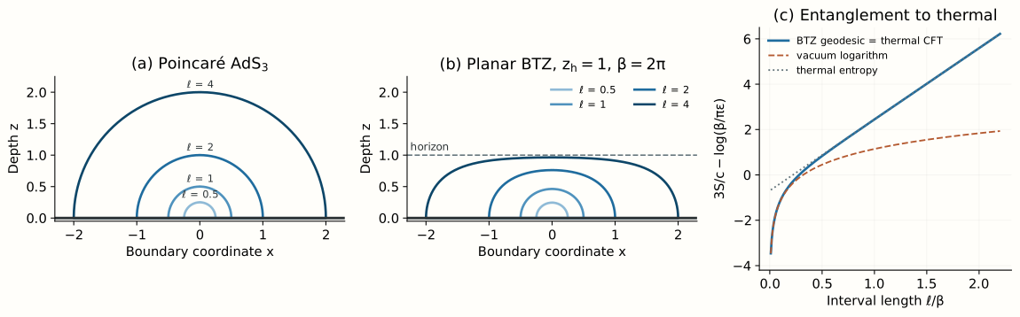
where $z_{\ast }$ is the turning point, at which $z^{\prime }=0$. Rearranging gives $dx/dz=z/\sqrt{z_{\ast }^2-z^2}$, and integration gives the semicircle $x^2+z^2=z_{\ast }^2$; the endpoints fix $z_{\ast }=R$ (Figure 1(a)). The depth reached by the geodesic is set by the size of the interval, the same relation between boundary scale and bulk depth that the propagator of Lecture 15 displayed.

To regulate the length, parametrize the semicircle by $x=R\cos \theta$, $z=R\sin \theta$, so that $d\mathcal{L}=Ld\theta /\sin \theta$, and cut it off at $z=ϵ$, that is at ${\theta }_{ϵ}=\arcsin (ϵ/R)$:

$${\mathcal{L}}_{ϵ}=2L\log \cot \frac{{\theta }_{ϵ}}{2}=2L\log \frac{R+\sqrt{R^2-{ϵ}^2}}{ϵ}=2L\log \frac{2R}{ϵ}+O\left(\frac{{ϵ}^2}{R^2}\right).$$

If instead one fixes the endpoints at $(\pm R,ϵ)$ before minimizing, the exact length is $2L\mathrm{arsinh}(R/ϵ)$. The two prescriptions agree in the leading logarithm and differ at order ${ϵ}^2/R^2$, which is a choice of cutoff.

5. Brown–Henneaux and the first match

With $\ell =2R$ the prescription gives

$$S_A=\frac{{\mathcal{L}}_{ϵ}}{4G_3}=\frac{L}{2G_3}\log \frac{\ell }{ϵ}+\dots .$$

Brown and Henneaux showed that the asymptotic symmetries of AdS${}_3$ form two Virasoro algebras with central charge (Lecture 12, Problem 15)

$$c=\frac{3L}{2G_3},$$

and with this value the geodesic gives $S_A=\frac{c}{3}\log (\ell /ϵ)$. [Exact match of the coefficient of the logarithm.] Note that the bulk calculation never used the replica trick or the twist fields, and the boundary calculation never used a metric. The agreement of the coefficients is the first test of the prescription; the constant term depends on the cutoff on each side and is not compared.

6. Finite temperature: the BTZ geodesic

The thermal state of a holographic CFT on an infinite line is dual, at every temperature, to the planar BTZ black hole; on a circle the same holds above the Hawking–Page temperature of Lecture 23. The planar geometry is

$$d{s}^2=\frac{L^2}{z^2}\left(-f(z)d{t}^2+\frac{d{z}^2}{f(z)}+d{x}^2\right),f(z)=1-\frac{z^2}{z_h^2},$$

whose Euclidean regularity at the horizon $z=z_h$ gives $\beta =4\pi /|f^{\prime }(z_h)|=2\pi z_h$. On a constant-time slice the length of a curve $z(x)$ is $L\int dx\sqrt{1+z^{\prime 2}/f}/z$, and the conserved Beltrami combination now reads

$$\frac{1}{z\sqrt{1+z^{\prime 2}/f(z)}}=\frac{1}{z_{\ast }}.$$

The half-width of the interval and the regulated length are then

$$\frac{\ell }{2}={\int }_0^{z_{\ast }}\frac{(z/z_{\ast })dz}{\sqrt{f(z)\left(1-z^2/z_{\ast }^2\right)}},{\mathcal{L}}_{ϵ}=2L{\int }_{ϵ}^{z_{\ast }}\frac{dz}{z\sqrt{f(z)\left(1-z^2/z_{\ast }^2\right)}}.$$

Both integrals are elementary (Problem 5). The first gives the turning point, $z_{\ast }=z_h\tanh (\ell /2z_h)$, and the second

$${\mathcal{L}}_{ϵ}=2L\log \left(\frac{2z_h}{ϵ}\sinh \frac{\ell }{2z_h}\right)+O({ϵ}^2)=2L\log \left(\frac{\beta }{\pi ϵ}\sinh \frac{\pi \ell }{\beta }\right)+O({ϵ}^2).$$

[Exact calculation.] Dividing by $4G_3$ and using $c=3L/2G_3$ reproduces the thermal result of §2.3 exactly, including its dependence on $\ell /\beta$.

The geometry of this agreement is instructive (Figure 1(b)). For $\ell \ll \beta$ the turning point is $z_{\ast }\simeq \ell /2$, and the geodesic is the semicircle of §4. As $\ell$ grows, $z_{\ast }$ approaches the horizon exponentially, $z_h-z_{\ast }\simeq 2z_h{e}^{-\ell /z_h}$, and the geodesic runs along the horizon for most of its length. The length of a horizon segment of coordinate width $\ell$ is $L\ell /z_h$, so the geodesic entropy approaches

$$\frac{L\ell }{4G_3{z}_h}=\frac{\pi c}{3}\frac{\ell }{\beta },$$

which is the Bekenstein–Hawking entropy of that segment of the horizon, and also the thermal entropy of the boundary segment. [Exact calculation.] The crossover from entanglement to thermal entropy in §2.3 is, in the bulk, the approach of the minimal surface to the horizon.

7. Why the prescription holds for balls

Casini, Huerta and Myers observed that for a ball in the vacuum of a CFT the entanglement entropy is a thermal entropy in disguise. Lecture 11 showed that the modular flow of a ball $B$ of radius $R$ is geometric, generated by a conformal Killing vector of its causal diamond. The same conformal transformation maps the diamond onto $\mathbb{R}\times H^{d-1}$, time times hyperbolic space of curvature radius $R$, and it maps the modular flow onto time translation. The vacuum restricted to the diamond therefore becomes the thermal state on hyperbolic space at

$$T=\frac{1}{2\pi R},$$

the temperature at which the modular parameter of Lecture 11 is physical time. The entanglement entropy of the ball equals the thermal entropy on $H^{d-1}$, with the ultraviolet cutoff at the boundary of the ball mapped to an infrared cutoff on the infinite volume of hyperbolic space. [Stated only — refs: Casini, Huerta, Myers; the conformal map follows from Lecture 11.]

In two dimensions every step can be carried out. The diamond of the interval $(-R,R)$ is conformal to the flat strip ${\mathbb{R}}_{\tau }\times {\mathbb{R}}_{\chi }$ with $\chi =R\log \frac{R+x}{R-x}$ on the slice $t=0$, the coordinate in which the modular flow of Lecture 11 is a translation. Cutting off at $|x|=R-ϵ$ gives a line of length $2R\log (2R/ϵ)$, up to terms of order $R$ that depend on how the cutoff is transported. On an infinite line a CFT at temperature $T$ has the entropy density $\frac{\pi c}{3}T$ of Lecture 12 exactly, because the map $z=e^{2\pi w/\beta }$ gives the energy density through the Schwarzian and thermodynamics gives the entropy, so

$$S_A=\frac{\pi c}{3}\cdot \frac{1}{2\pi R}\cdot 2R\log \frac{2R}{ϵ}+O(1)=\frac{c}{3}\log \frac{2R}{ϵ}+O(1),$$

which is the interval entropy of §2.3 with $\ell =2R$. [Exact calculation, up to the constant.]

In the bulk, the thermal state on $\mathbb{R}\times H^{d-1}$ at $T=1/(2\pi R)$ is dual to a hyperbolic black hole whose metric is AdS itself in AdS-Rindler coordinates. Its horizon is the extremal surface anchored on the boundary of the ball, the hemisphere of the Poincaré patch, and the thermal entropy of the boundary theory is the Bekenstein–Hawking entropy of that horizon. For $d=2$ the horizon is the semicircle of §4 and its length gives the same logarithm. The Ryu–Takayanagi formula for balls thus follows from a property of the CFT, the conformal map, combined with holographic input: the identification of the thermal state on hyperbolic space with the hyperbolic black hole, whose entropy is the Bekenstein–Hawking entropy of its horizon. Nevertheless the argument uses the geometric modular flow of balls, and for general regions the modular Hamiltonian is nonlocal; the general derivation requires the replica argument of Lewkowycz and Maldacena (§8 and Lecture 27).

8. Homology, the plateau, and the covariant prescription

Anchoring alone says only where the surface ends. The homology condition requires that $A$ and ${\gamma }_A$ together bound a region of the bulk slice, which becomes the spatial part of the entanglement wedge of Lecture 19. For a single interval in the Poincaré vacuum the condition is automatic: the semicircle and the interval bound a half-disk.

In the presence of a horizon the condition does real work. Consider the thermal state on a circle, dual to the global BTZ black hole, and an interval $A$ with complement $\bar{A}$. There are two candidate surfaces homologous to $\bar{A}$: the geodesic anchored on its endpoints that passes on the other side of the horizon, and the geodesic of $A$ together with the horizon itself. For a small $\bar{A}$ the first is shorter. For a large $\bar{A}$ the second is, and then

$$S_{\bar{A}}=S_A+S_{\mathrm{BH}},$$

which saturates the Araki–Lieb inequality $|S_A-S_{\bar{A}}|\le S(\rho )$ with the thermal entropy $S(\rho )=S_{\mathrm{BH}}$. This is the entanglement plateau of Hubeny, Maxfield, Rangamani and Tonni. [Exact within the prescription.] Without the homology condition, the geodesic of $A$ alone would be a candidate for $\bar{A}$ and would give $S_A=S_{\bar{A}}$, the relation of a pure state, which the thermal state is not.

A time-dependent geometry has no preferred static slice. The covariant prescription of Hubeny, Rangamani and Takayanagi uses codimension-two surfaces that are extremal in spacetime, anchored and homologous, and selects among them the one of smallest area. A Lorentzian area functional is not minimized over all deformations: a spatial geodesic is a minimum under spatial variations and a maximum under variations in a timelike direction. Wall’s maximin construction and the explicit Lorentzian extremum of Lecture 26 make the selection precise. With quantum fields in the bulk, Engelhardt and Wall proposed extremizing the generalized entropy $\mathrm{Area}/4G_N+S_{\mathrm{bulk}}$ in place of the area, which defines the quantum extremal surface. Its leading approximation, when the area term dominates, is the classical extremal surface with the bulk entropy of Faulkner, Lewkowycz and Maldacena evaluated on it. Lewkowycz and Maldacena derived the static prescription from the gravitational replica trick. The $n$-fold boundary condition is filled in by a bulk geometry whose quotient by the replica symmetry has a conical defect, and as $n\to 1$ the defect settles on the extremal surface; Dong, Lewkowycz and Rangamani later extended the argument to the covariant case. [Sketched here; Lecture 27 develops it.]

9. Self-study: what the code analogy captures

In a code with a fixed sector structure, the entanglement of a region with an auxiliary system contributes a term that is the same for every logical state in a sector (Lecture 4). In gravity the area term plays that role at order $1/G_N$, and the central operator of Lecture 4 becomes the area operator of Lecture 21. This is a structural analogy with a precise algebraic realization. A graph edge count equals a smooth area only after additional modeling assumptions. Changing the bond weights of a tensor network can lower its entropy without changing the drawn cut, as Lecture 6 showed, and higher-derivative gravity changes the entropy functional itself. The Einstein area formula is the leading term in the regime of Lecture 14.

10. What to take away

• Exact: the Schwarzian fixes the twist-field dimension ${\Delta }_n=\frac{c}{12}(n-\frac{1}{n})$, and the interval entropy is $\frac{c}{3}\log (\ell /ϵ)$; conformal maps give $\frac{c}{3}\log \left(\frac{\beta }{\pi ϵ}\sinh \frac{\pi \ell }{\beta }\right)$ at finite temperature.
• Stated only: the Ryu–Takayanagi prescription, $S_A=\mathrm{Area}({\gamma }_A)/4G_N$ at leading order in a holographic CFT, with the homology condition.
• Exact: the Poincaré and BTZ geodesics reproduce both CFT results with $c=3L/2G_3$, including the crossover to the thermal entropy, where the geodesic runs along the horizon.
• Exact on the CFT side, holographic in the bulk: the entanglement entropy of a ball is a thermal entropy on hyperbolic space, exactly so in $d=2$; holographically it is the Bekenstein–Hawking entropy of the AdS-Rindler horizon.
• Exact within the prescription: homology produces the entanglement plateau $S_{\bar{A}}=S_A+S_{\mathrm{BH}}$ in a thermal state; covariantly the surface is extremal, and quantum corrections add the bulk entropy.

11. Looking ahead

Lecture 17 connects the finite codes of the opening block with the geometric entropy of this lecture. Lecture 18 asks which bulk operators can be reconstructed from the boundary region, and Lecture 19 uses the region bounded by the minimal surface, the entanglement wedge, with the two-interval transition that the homology condition makes possible. Lecture 22 returns to the ball of §7 and derives the linearized Einstein equations from the first law of entanglement.

12. Problem set

Classroom core

1. The replica stress tensor. Using the composition law of the Schwarzian, derive $⟨T(z){⟩}_{{\mathcal{R}}_n}$ and the twist-field dimension $h_n$.

2. Maps to the cylinder. Derive the thermal and finite-size interval entropies of §2.3 from the transformation of the twist fields under $z=e^{2\pi w/\beta }$ and $z=e^{2\pi iw/L_c}$.

3. Rényi entropies. Compute $S_n$ from $\mathrm{Tr}{\rho }_A^n$, and check that $S_{\infty }=\frac{c}{6}\log (\ell /ϵ)$ is half of $S_1$. What does $S_{\infty }$ measure?

4. The semicircle. Integrate the Beltrami equation of §4, and compare the two cutoff prescriptions to order ${ϵ}^2/R^2$.

5. The BTZ geodesic. Evaluate the two integrals of §6 with the substitution $z=z_{\ast }\sin \theta$, and derive $z_{\ast }=z_h\tanh (\ell /2z_h)$ and the regulated length.

6. The thermal limit. Expand the BTZ entropy at large $\ell /\beta$ and identify the leading term with the Bekenstein–Hawking entropy of a segment of the horizon.

Self-study consolidation

7. Strong subadditivity. For three adjacent intervals of lengths $a,b,c$ in the vacuum, show that $S(AB)+S(BC)\ge S(B)+S(ABC)$. Repeat at finite temperature using the concavity of $\log \sinh$.

8. Units. Why is $\mathcal{L}/(4G_3)$ dimensionless in three dimensions?

9. A wrong network inference. A cut crosses two bonds of dimension $D$. Is the entropy of the region necessarily $2\log D$?

10. The hyperbolic line. Derive $\chi =R\log \frac{R+x}{R-x}$ from the modular flow of Lecture 11, and show that the modular parameter becomes physical time at $T=1/(2\pi R)$.

11. The circle. Show that the vacuum entropy on a circle is symmetric under $\ell \mapsto L_c-\ell$, and find the geodesic in global AdS${}_3$ that reproduces it.

12. The plateau. In global BTZ with boundary circumference $L_c$, find the critical length ${\ell }_{\ast }$ of $A$ below which the entropy of $\bar{A}$ is given by the geodesic of $A$ together with the horizon.

Research extension

13. The gravitational replica trick. Follow Lewkowycz and Maldacena to derive the extremality condition from the regularity of the replica geometry near $n=1$. Known: their paper and Lecture 27. Completion: the conical-defect tension $(n-1)/(4n{G}_N)$ and the extremal-surface equation from the $n\to 1$ limit.

14. Quantum corrections. Estimate the displacement of the extremal surface produced by a bulk entropy term for a nondegenerate classical extremum. Known: the Faulkner–Lewkowycz–Maldacena correction and the quantum extremal surface of Engelhardt and Wall. Completion: the displacement as the inverse area Hessian acting on the gradient of the bulk entropy, and a case in which the estimate fails.

15. Holographic proof of strong subadditivity. Reproduce the cut-and-paste argument of Headrick and Takayanagi for static geometries. Known: their paper. Completion: the argument for three adjacent intervals in AdS${}_3$, and an explanation of what fails for time-dependent geometries without the maximin construction.

13. Answer checkpoints

1. Write $w={\zeta }^{1/n}$ with $\zeta =(z-u)/(z-v)$. The composition law gives $\{w,z\}=\{w,\zeta \}(d\zeta /dz{)}^2+\{\zeta ,z\}$, where $\{\zeta ,z\}=0$ for a Möbius map, $\{{\zeta }^{1/n},\zeta \}=(1-n^{-2})/(2{\zeta }^2)$ and $d\zeta /dz=(u-v)/(z-v{)}^2$. Multiplying by $c/12$ and by $n$ sheets, and comparing with the Ward identity, gives $h_n=\frac{c}{24}(n-\frac{1}{n})$.

2. For the thermal map, $|dz/dw|=\frac{2\pi }{\beta }|z|$, and endpoints at $w=0$ and $w=\ell$ give $|z_1^{\prime }||z_2^{\prime }|/|z_1-z_2{|}^2=(\pi /\beta {)}^2/{\sinh }^2(\pi \ell /\beta )$. The twist two-point function is this ratio to the power ${\Delta }_n$, and differentiating at $n=1$ gives the entropy. For the circle the same steps with $z=e^{2\pi iw/L_c}$ replace $\sinh$ by $\sin$.

3. $S_n=\frac{1}{1-n}\cdot \left(-\frac{c}{6}\right)\left(n-\frac{1}{n}\right)\log \frac{\ell }{ϵ}=\frac{c}{6}\left(1+\frac{1}{n}\right)\log \frac{\ell }{ϵ}$. As $n\to \infty$ this is $\frac{c}{6}\log (\ell /ϵ)$, half of $S_1$. The min-entropy $S_{\infty }=-\log {\lambda }_{\max }$ measures the largest eigenvalue of ${\rho }_A$.

4. $x^2+z^2=z_{\ast }^2$ with $z_{\ast }=R$. The first prescription gives $2L\log \frac{2R}{ϵ}-\frac{L{ϵ}^2}{2R^2}+\dots$, and $2L\mathrm{arsinh}(R/ϵ)=2L\log \frac{2R}{ϵ}+\frac{L{ϵ}^2}{2R^2}+\dots$; the leading terms agree.

5. With $z=z_{\ast }\sin \theta$, the width integral becomes ${\int }_0^{\pi /2}\frac{z_{\ast }\sin \theta d\theta }{\sqrt{1-(z_{\ast }^2/z_h^2){\sin }^2\theta }}$, which equals $z_h\mathrm{artanh}(z_{\ast }/z_h)$, so $\ell /2=z_h\mathrm{artanh}(z_{\ast }/z_h)$. The length integral gives $2L\log \left(\frac{2z_{\ast }}{ϵ\sqrt{1-z_{\ast }^2/z_h^2}}\right)$ up to $O({ϵ}^2)$, and substituting $z_{\ast }=z_h\tanh (\ell /2z_h)$ gives $2L\log \left(\frac{2z_h}{ϵ}\sinh \frac{\ell }{2z_h}\right)$.

6. $\log \sinh x=x-\log 2+O(e^{-2x})$, so $S\simeq \frac{c}{3}\frac{\pi \ell }{\beta }+\frac{c}{3}\log \frac{\beta }{2\pi ϵ}$. The first term equals $L\ell /(4G_3{z}_h)$, the length of the horizon segment divided by $4G_3$.

7. In the vacuum the inequality is $\log (a+b)+\log (b+c)\ge \log b+\log (a+b+c)$, equivalent to $(a+b)(b+c)-b(a+b+c)=ac\ge 0$. At finite temperature the same inequality for $\log \sinh (\pi \cdot /\beta )$ follows from its concavity.

8. In three dimensions $G_3$ has units of length when $\hslash =c=1$, and $\mathcal{L}$ is a length.

9. No. It is an upper bound; saturation requires a flat Schmidt spectrum across the cut and the isometric properties of Lecture 6.

10. Lecture 11 found that $u^{\pm }=\log \frac{R+x^{\pm }}{R-x^{\pm }}$ translate by $2\pi s$ under modular flow. With $\tau =R(u^{+}+u^{-})/2$ and $\chi =R(u^{+}-u^{-})/2$, modular flow is $\tau \mapsto \tau +2\pi Rs$, so the KMS period $s\mapsto s+i$ is an imaginary time $2\pi R$, a temperature $1/(2\pi R)$. At $t=0$, $u^{-}=-u^{+}$ and $\chi =R\log \frac{R+x}{R-x}$.

11. $\sin (\pi \ell /L_c)$ is invariant under $\ell \mapsto L_c-\ell$. In global AdS${}_3$ a unique geodesic joins two boundary points separated by an angle $2\pi \ell /L_c$, with regulated length $2L\log \left(\frac{L_c}{\pi ϵ}\sin \frac{\pi \ell }{L_c}\right)$. Because the slice has no horizon, that geodesic is homologous to both $A$ and $\bar{A}$, which is the bulk statement of $S_A=S_{\bar{A}}$ in a pure state.

12. The two candidates for $\bar{A}$ have entropies $\frac{c}{3}\log \left(\frac{\beta }{\pi ϵ}\sinh \frac{\pi (L_c-\ell )}{\beta }\right)$ and $\frac{c}{3}\log \left(\frac{\beta }{\pi ϵ}\sinh \frac{\pi \ell }{\beta }\right)+\frac{\pi c}{3}\frac{L_c}{\beta }$, in the high-temperature phase where the horizon entropy is Cardy’s. They are equal when $\sinh \frac{\pi (L_c-\ell )}{\beta }=e^{\pi L_c/\beta }\sinh \frac{\pi \ell }{\beta }$, whose solution is ${\ell }_{\ast }=\frac{\beta }{2\pi }\log \frac{2}{1+e^{-2\pi L_c/\beta }}$, close to $\frac{\beta }{2\pi }\log 2$ when $L_c\gg \beta$. For $\ell <{\ell }_{\ast }$ the second candidate is smaller.

13. Guide. Assume replica symmetry, pass to the quotient geometry, and expand the action near $n=1$. The fixed points of the replica symmetry carry a cosmic brane of tension $(n-1)/(4n{G}_N)$, whose back-reaction vanishes at $n=1$; stationarity of the action with respect to the brane position is the extremality condition, and the derivative of the action at $n=1$ is the area over $4G_N$.

14. Guide. Expand $\mathrm{Area}/4G_N+S_{\mathrm{bulk}}$ around the classical extremum. The displacement is $\delta X=-4G_N{H}^{-1}\nabla S_{\mathrm{bulk}}$ with $H$ the second variation of the area, of order $G_N$. Near a zero mode of $H$ or a transition between competing surfaces the expansion fails.

15. Guide. The minimal curves for $AB$ and $BC$ cross; exchanging their pieces at the crossing produces two curves anchored on $B$ and on $ABC$, which are not minimal, so their lengths bound $S(B)+S(ABC)$ from above by $S(AB)+S(BC)$. For time-dependent geometries the surfaces need not lie on a common slice, and the maximin construction provides one.

Wiki connections. Ryu–Takayanagi formula · causal diamonds