Lecture 17 — From a recoverable observable to a geometric region

The first semester asked four questions about a region: which observables it gives access to, which states it can tell apart, what it can recover, and how its entropy and its modular flow are organized. This lecture puts the answers side by side in the two examples that carried the semester. In the three-qutrit code of Lecture 2 the answers are exact. A single share knows nothing, a pair recovers everything, and the entropy of the pair exceeds that of the logical state by $\log 3$, an auxiliary entanglement that drops out of relative entropy and of the modular flow. The code with sectors of Lecture 4 lets that term vary with the state, and the first law then contains it, as the first law of holography contains the change of an area. In the vacuum of a two-dimensional conformal field theory, an interval has a geometric modular flow (Lecture 11) and, in a holographic theory, an entropy equal to the length of a geodesic divided by $4G_3$ (Lecture 16). We compute the first law of a thermal perturbation twice, as the modular energy of the boundary stress tensor and as the change of the geodesic’s length under the change of the metric, and obtain the same number. In the coordinates of the BTZ metric the two integrands differ point by point; in Fefferman–Graham coordinates, where the metric perturbation is the holographic stress tensor, they coincide, and the coincidence is the linearized Hamiltonian constraint of Lecture 22. The lecture ends by auditing an overstated argument and by stating the questions that the second semester answers.

How to use this lecture

Classroom core, two meetings of two hours. The first meeting covers what the semester connected (§1, 10 minutes), the four questions in the three-qutrit code (§2, 35 minutes), the modular flow and the first law of a recovering pair (§3, 30 minutes), and a varying central term (§4, 30 minutes), leaving 15 minutes for Checkpoints 1 and 2. The second meeting covers the vacuum interval in three descriptions (§5, 25 minutes), the first law as a property of a geodesic (§6, 35 minutes), what the comparison carries (§7, 20 minutes), and the audit of an argument (§8, 15 minutes), with 25 minutes for Problems 1–4; Problems 5 and 6 complete the core assignment. These allocations are proposals and have not been tested in class.

Self-study. The derivation chain of the semester (§9), the questions of the second semester (§10), and Problems 7–12, including negative conditional entropy, the energy density from Cardy’s formula, the second-order deficit of the geodesic and the cutoff independence of the entropy difference.

Research extension. The first law in heavy states, positivity of relative entropy as a bulk energy condition, and a code whose central term fluctuates, in Problems 13–15.

Prerequisites. Lecture 2 for the three-qutrit code and its decoder, Lecture 3 for modular Hamiltonians, Lecture 4 for codes with sectors, Lecture 11 for the modular flow of an interval and the first law, Lecture 12 for Cardy’s formula, Lecture 16 for the interval entropy and the Poincaré and BTZ geodesics. Relative entropy, modular Hamiltonians and the Ryu–Takayanagi prescription.

What this lecture establishes. The four answers of the three-qutrit code, the modular Hamiltonian of a recovering pair with the cancellation of its auxiliary term in modular flow and relative entropy, the first law of a code with a varying central term, and the first-order variation of the length of the BTZ geodesic, which equals the modular energy of the thermal interval and, in Fefferman–Graham gauge, equals it point by point, are exact calculations or proofs. The Ryu–Takayanagi prescription, the conformal modular flow of the interval and the holographic meaning of the positivity of relative entropy are stated with sources.

0. Reading

Primary.

• A. Almheiri, X. Dong, D. Harlow, Bulk Locality and Quantum Error Correction in AdS/CFT (2014).
• D. D. Blanco, H. Casini, L.-Y. Hung, R. C. Myers, Relative Entropy and Holography (2013).
• H. Casini, M. Huerta, R. C. Myers, Towards a derivation of holographic entanglement entropy (2011).

Secondary.

• D. Harlow, The Ryu-Takayanagi Formula from Quantum Error Correction (2016).
• D. Harlow, TASI Lectures on the Emergence of the Bulk in AdS/CFT (2018).
• R. Cleve, D. Gottesman, H.-K. Lo, How to share a quantum secret (1999).

Optional research reading.

• J. Lin, M. Marcolli, H. Ooguri, B. Stoica, Tomography from Entanglement (2014).
• N. Lashkari, M. Van Raamsdonk, Canonical Energy is Quantum Fisher Information (2015).
• C. T. Asplund, A. Bernamonti, F. Galli, T. Hartman, Holographic Entanglement Entropy from 2d CFT: Heavy States and Local Quenches (2014).

1. What did the first semester connect?

The semester drew on three lines of work that met around 2014. The algebraic line begins with the local algebras of Haag and Kastler in 1964, the modular theory of Tomita and Takesaki around 1970, the theorem of Bisognano and Wichmann of 1975, which made the vacuum modular flow of a wedge a boost, and Araki’s relative entropy of 1976; in 1982 Hislop and Longo found the conformal modular flow of a ball for the free massless scalar, and Brunetti, Guido and Longo extended it to conformal nets in 1993 (Lectures 3 and 9–11). The holographic line runs from the central charge of Brown and Henneaux in 1986 and Maldacena’s conjecture of 1997 to the formula of Ryu and Takayanagi in 2006, which Casini, Huerta and Myers explained for balls in 2011 by mapping the causal diamond to hyperbolic space, where the entanglement entropy becomes a thermal entropy and, holographically, the entropy of a horizon (Lectures 12–16). The information line begins with Shor’s error-correcting code of 1995 and with quantum secret sharing, whose three-qutrit scheme Cleve, Gottesman and Lo published in 1999 (Lecture 2).

The lines met in two papers. In 2013 Blanco, Casini, Hung and Myers showed that the first law of entanglement, which holographic calculations had found for small excitations, is the first-order vanishing of a relative entropy. In 2014 Almheiri, Dong and Harlow recognized the three-qutrit code in the reconstruction of a bulk point from several boundary regions. In 2015 Pastawski, Yoshida, Harlow and Preskill built tensor-network codes with complementary recovery and a cut formula (Lecture 6), and in 2016 Harlow proved that complementary recovery is equivalent to an entropy formula with a central area term, for a region and its complement (Lectures 4 and 21). This lecture follows the meeting of the lines in the two examples where every step can be computed.

2. One encoded qutrit and four questions

Recall the encoding of Lecture 2,

$$V|i⟩=\frac{1}{\sqrt{3}}\sum _{r=0}^2|r,r+i,r+2i⟩,$$

with labels modulo three, and a faithful logical state $\rho$. We ask the four questions of the semester of a single share, of a pair and of all three shares.

What can a region measure? A single share has the reduced state $I_3/3$ for every logical input (Lecture 2, §3). Every observable of one share has the same expectation value in every encoded state, so the share carries no logical information at all.

What can it recover? The pair $(1,2)$ has a decoder, a unitary $D_{12}$ on the two shares, that maps the state of the pair to the logical state times a fixed auxiliary state,

$$D_{12}{\rho }_{12}{D}_{12}^{†}=\rho \otimes \frac{I_3}{3},$$

where the auxiliary qutrit is maximally entangled with the third share (Lecture 2, §4). Every logical operator $O$ then has a representative on the pair, $O_{12}=D_{12}^{†}(O\otimes I)D_{12}$, and so does every logical operator on each of the other two pairs. No two disjoint regions can both carry it (Lecture 2, §5.2, the operator form of the no-cloning argument of §7).

What can it distinguish? For two logical states $\rho$ and $\sigma$, the auxiliary factor is the same, so

$$D({\rho }_1\Vert {\sigma }_1)=0,D({\rho }_{12}\Vert {\sigma }_{12})=D(\rho \otimes \frac{I_3}{3}\Vert \sigma \otimes \frac{I_3}{3})=D(\rho \Vert \sigma ),D({\rho }_{123}\Vert {\sigma }_{123})=D(\rho \Vert \sigma ),$$

the last because an isometry preserves relative entropy.

What is its entropy? The same three facts give

$$S({\rho }_1)=\log 3,S({\rho }_{12})=S(\rho )+\log 3,S({\rho }_{123})=S(\rho ).$$

[Exact calculation (Lecture 2).] A single share has the largest entropy per qutrit and no information; the pair has more entropy than the whole, so that $S(123)-S(12)=-\log 3<0$, a negative conditional entropy that no classical system allows (Problem 7). For $\rho =\mathrm{diag}(0.7,0.2,0.1)$ and $\sigma =I_3/3$ the numbers are $S(\rho )=0.80$, $S({\rho }_1)=1.10$, $S({\rho }_{12})=1.90$ and $D(\rho \Vert \sigma )=\log 3-S(\rho )=0.30$, in nats; figure (a) shows them.

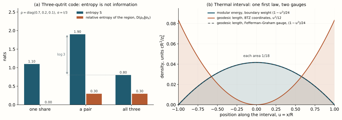
The four answers already separate two notions that the second semester keeps apart: entropy measures how mixed the state of a region is, and relative entropy measures what the region knows about the logical state. The single share maximizes the first and has none of the second.

3. Modular flow and the first law of a recovering pair

Take a faithful logical reference $\sigma$, with one-sided modular Hamiltonian $K_{\sigma }=-\log \sigma$ in the sense of Lecture 3, §4. Since ${\sigma }_{12}=D_{12}^{†}(\sigma \otimes I_3/3)D_{12}$, the decoder gives

$$K_{12}=-\log {\sigma }_{12}=D_{12}^{†}(K_{\sigma }\otimes I+\log 3I\otimes I)D_{12}.$$

The constant $\log 3$ is the modular Hamiltonian of the auxiliary state $I_3/3$. It commutes with everything, so the modular flow of a recovered operator is the logical modular flow,

$$e^{is{K}_{12}}{O}_{12}{e}^{-is{K}_{12}}=D_{12}^{†}(e^{is{K}_{\sigma }}O{e}^{-is{K}_{\sigma }}\otimes I)D_{12},$$

and for a diagonal $\sigma =\mathrm{diag}(q_0,q_1,q_2)$ and $O=|i⟩⟨j|$ the flow is multiplication by $e^{is\log (q_j/q_i)}$. [Exact calculation.] The modular frequencies are logarithms of ratios of reference weights; they are $\beta$ times the Bohr frequencies $E_i-E_j$ of a Hamiltonian $H$ only when the reference is the Gibbs state of $H$, as Lecture 3, §6 showed.

The first law follows at once. For $\rho =\sigma +\delta \rho$,

$$\delta S({\rho }_{12})=\delta S(\rho )=\mathrm{Tr}(\delta \rho K_{\sigma })+O(\delta {\rho }^2)=\delta ⟨K_{12}⟩+O(\delta {\rho }^2),$$

since the auxiliary term contributes $\log 3\mathrm{Tr}\delta \rho =0$. The difference of the two sides at finite $\delta \rho$ is the relative entropy, $\Delta ⟨K_{12}⟩-\Delta S({\rho }_{12})=D({\rho }_{12}\Vert {\sigma }_{12})=D(\rho \Vert \sigma )$, nonnegative and of second order in $\delta \rho$. [Proved: the equality of relative entropies in Lecture 4, §6.1; $D=\Delta ⟨K⟩-\Delta S\ge 0$ and the first law as its stationarity in Lecture 11, §6.] The first law is the stationarity of a nonnegative function at its minimum, and the auxiliary entanglement plays no role in it.

Physical picture: an area term is entanglement that the encoding supplies. The auxiliary qutrit of the pair is maximally entangled with the third share, whatever the logical state. An observer of the pair sees that entanglement as a fixed amount of entropy, $\log 3$, which no logical operation changes. It enters the entropy of the pair and leaves every comparison of two states, because both states carry it. In holography the area of a surface behaves the same way at the order at which it is a fixed number; when it changes with the state, it does so as a central operator, which the next section models.

4. A varying central term

The two-qutrit code of Lecture 4, §8, makes the central term depend on the state. A logical qubit is encoded as

$$V|0⟩=|0,0⟩,V|1⟩=\frac{1}{\sqrt{2}}(|1,1⟩+|2,2⟩),$$

and each qutrit recovers the diagonal algebra $\mathcal{M}=\mathrm{span}\{P_0,P_1\}$. For a logical state with sector probabilities $p$ and $1-p$, each side has the reduced state ${\tilde{\rho }}_A=\mathrm{diag}(p,\frac{1-p}{2},\frac{1-p}{2})$, and

$$S({\tilde{\rho }}_A)=h(p)+(1-p)\log 2=S_{\mathcal{M}}(\rho )+⟨{\mathcal{L}}_A{⟩}_{\rho },{\mathcal{L}}_A=(\log 2)P_1,$$

with $h$ the binary entropy. [Exact calculation (Lecture 4, §8).] The central operator ${\mathcal{L}}_A$ counts the entangled pair that sector $1$ contains and sector $0$ does not.

Now perturb the reference $q$ to $p=q+\delta p$. The entropy changes by

$$\delta S({\tilde{\rho }}_A)=[\log \frac{1-q}{q}-\log 2]\delta p=\delta S_{\mathcal{M}}+\delta ⟨{\mathcal{L}}_A⟩,$$

and the modular Hamiltonian of the reference, $K_A=-\log {\tilde{\sigma }}_A=\mathrm{diag}(-\log q,-\log \frac{1-q}{2},-\log \frac{1-q}{2})$, has

$$\delta ⟨K_A⟩=\mathrm{Tr}\left(\delta {\tilde{\rho }}_A{K}_A\right)=[-\log q+\log \frac{1-q}{2}]\delta p=\delta S({\tilde{\rho }}_A).$$

[Exact calculation (Problem 4).] The first law holds, and the area term contributes $-\log 2\delta p$ to it: when the probability of the sector with the entangled pair decreases, the entropy loses the corresponding amount of entanglement. On the code the modular Hamiltonian is $V^{†}{K}_{A}V=K_{\mathcal{M}}+{\mathcal{L}}_A$, with $K_{\mathcal{M}}=-\log q{P}_0-\log (1-q)P_1$, so the central term appears in the modular energy with the same coefficient as in the entropy, and the relative entropy does not contain it,

$$D({\tilde{\rho }}_A\Vert {\tilde{\sigma }}_A)=p\log \frac{p}{q}+(1-p)\log \frac{1-p}{1-q}=D_{\mathcal{M}}(\rho \Vert \sigma ).$$

[Exact calculation (Lecture 4, §8.3).] Here $\mathcal{M}$ is abelian, and its modular flow is trivial; the statement that a central term drops out of the modular flow has content when the sectors carry matrix algebras, as in Lecture 21.

These identities hold in every code with sectors and fixed auxiliary states: $S({\rho }_A)=⟨{\mathcal{L}}_A{⟩}_{\rho }+S_{\mathcal{M}}(\rho )$ with ${\mathcal{L}}_A$ central, $V^{†}{K}_{A}V=K_{\mathcal{M}}+{\mathcal{L}}_A$, and $D({\rho }_A\Vert {\sigma }_A)=D_{\mathcal{M}}(\rho \Vert \sigma )$. [Proved (Lectures 4 and 21).] They are the finite form of the relation of Jafferis, Lewkowycz, Maldacena and Suh, which Lecture 21 develops, in which ${\mathcal{L}}_A$ becomes the area operator divided by $4G_N$.

Checkpoint 1. In the two-qutrit code, why does the central term contribute to the first law while cancelling from the relative entropy?

Answer. Its expectation value changes at first order when the sector probabilities change, so it enters $\delta S$. Relative entropy is $\Delta ⟨K_A⟩-\Delta S$, and ${\mathcal{L}}_A$ appears in $K_A$ and in $S$ with the same coefficient, so it cancels.

Checkpoint 2. The constant $\log 3$ of §3 and the operator ${\mathcal{L}}_A$ of §4 both drop out of the modular flow of the recovered algebra. Why, when one is a number and the other is not?

Answer. A multiple of the identity commutes with every operator, and a central element commutes with every element of $\mathcal{M}$. In both cases the term commutes with the recovered algebra, so it does not affect the conjugation $e^{isK}\cdot e^{-isK}$ on that algebra. In the two-qutrit code $\mathcal{M}$ is abelian and the flow is trivial in any case; the three-qutrit pair, whose recovered algebra is all of $M_3(\mathbb{C})$, and the sector codes of Lecture 21 are where the statement has content.

5. The vacuum interval in three descriptions

Consider the interval $A=(-R,R)$ in the vacuum of a two-dimensional conformal field theory with $c=\bar{c}$. Three descriptions of it were developed in the semester.

The modular flow. The vacuum modular flow of the interval is the conformal flow that fixes its endpoints, and the modular Hamiltonian is local,

$$K_A=2\pi {\int }_{-R}^{R}dx\frac{R^2-x^2}{2R}{T}_{00}(x)+\text{const},$$

the conformal image of the boost of Lecture 10. [Stated only, with a sketch in Lecture 11 — refs: Hislop–Longo 1982; Brunetti–Guido–Longo 1993.]

The entropy. The twist fields of Lecture 16, §2, give $S_A=\frac{c}{3}\log \frac{2R}{ϵ}+s_0$, with $ϵ$ the cutoff at the endpoints and $s_0$ a nonuniversal constant. [Exact calculation in the CFT.]

The geodesic. In Poincaré AdS${}_3$ the geodesic anchored at the endpoints is the semicircle $x^2+z^2=R^2$, of regulated length $2L\log (2R/ϵ)$ (Lecture 16, §4), and with $c=3L/2G_3$ its length divided by $4G_3$ reproduces the coefficient $c/3$ of the logarithm. [Exact match of the coefficient of the logarithm; the constants depend on the cutoffs and are not compared; the Ryu–Takayanagi prescription is stated.] Casini, Huerta and Myers explained the match for balls. The causal diamond of the interval is conformal to time times a hyperbolic line, on which the vacuum is thermal at temperature $1/2\pi R$; the entanglement entropy is a thermal entropy, and in the bulk it is the entropy of the horizon of the AdS–Rindler wedge, whose bifurcation surface is the geodesic (Lecture 16, §7). [Stated only — refs: Casini–Huerta–Myers 2011; the bulk step is holographic input.] The bulk extension of the modular flow, whose generating Killing vector vanishes on the geodesic, is the subject of Lecture 22, §4.

The three descriptions share the cutoff term. The divergent part of the entropy, the term $\frac{c}{3}\log (1/ϵ)$, comes from the endpoints of the interval and, in the bulk, from the part of the geodesic near the boundary. It is the same in every state whose energy density is finite, and it drops out of every difference of entropies, as $\log 3$ drops out in the code.

6. The first law as a property of a geodesic

Heat the theory to a small temperature $T=1/\beta$. On the boundary, the energy density rises by $\Delta \mathcal{E}=\pi c{T}^2/6$, which follows from Cardy’s entropy density $\pi cT/3$ of Lecture 12, §8.4, through $d\mathcal{E}=Td(\pi cT/3)$ (Problem 8). The modular energy of the interval changes by

$$\Delta ⟨K_A⟩=2\pi \Delta \mathcal{E}{\int }_{-R}^{R}dx\frac{R^2-x^2}{2R}=\frac{2{\pi }^{2}c}{9}{R}^2{T}^2,$$

as Lecture 11, §8, found. [Exact calculation.]

In the bulk, the thermal state is the planar BTZ geometry of Lecture 16, §6, whose constant-time slice has the metric

$$d{s}^2=\frac{L^2}{z^2}\left(\frac{d{z}^2}{f(z)}+d{x}^2\right),f(z)=1-\frac{z^2}{z_h^2},z_h=\frac{\beta }{2\pi }.$$

In these coordinates, at first order in $1/z_h^2$, the only change of the slice metric is $\delta g_{zz}=L^2/z_h^2$, a constant. The geodesic is extremal with fixed endpoints, so the change of its shape does not change its length at first order, and the first-order change of the length ${\ell }_{\gamma }$ is the change of the metric integrated along the unperturbed curve,

$$\delta {\ell }_{\gamma }=\frac{1}{2}\int ds\delta g_{ab}\frac{d{x}^a}{ds}\frac{d{x}^b}{ds}.$$

On the semicircle $z=R\sin \theta$, $x=R\cos \theta$, the vacuum line element is $ds=Ld\theta /\sin \theta$ and $dz/ds=R\cos \theta \sin \theta /L$. Therefore

$$\delta {\ell }_{\gamma }=\frac{1}{2}{\int }_0^{\pi }\frac{Ld\theta }{\sin \theta }\frac{L^2}{z_h^2}\frac{R^2{\cos }^2\theta {\sin }^2\theta }{L^2}=\frac{L{R}^2}{2z_h^2}{\int }_0^{\pi }{\cos }^2\theta \sin \theta d\theta =\frac{L{R}^2}{3z_h^2},$$

and with $c=3L/2G_3$ and $z_h=1/2\pi T$,

$$\delta S_A=\frac{\delta {\ell }_{\gamma }}{4G_3}=\frac{c}{18}\frac{R^2}{z_h^2}=\frac{2{\pi }^{2}c}{9}{R}^2{T}^2=\Delta ⟨K_A⟩.$$

[Exact calculation of the first-order coefficient, given the Ryu–Takayanagi prescription; checked symbolically.] The integrand behaves as $(L/2z_h^2)zdz$ near the boundary, so the integral converges and the cutoff can be removed; a change of the radial coordinate at order $z^3/z_h^2$ moves the cutoff surface and changes the length only at order ${ϵ}^2$. The first law of entanglement holds, and on the bulk side it is a statement about how a geodesic responds to a change of the metric.

Both sides are integrals over the interval, and their integrands can be compared. In units of $c{R}^2/z_h^2$ and with $u=x/R$, the modular energy is ${\int }_{-1}^{1}du(1-u^2)/24$, a boundary weight largest at the center of the interval, where the modular flow is fastest. In the coordinates of the displayed metric the length is ${\int }_{-1}^{1}du{u}^2/12$, a weight largest near the endpoints: per unit $u$ the proper length $Ldu/(1-u^2)$ grows toward the endpoints while the fractional change $\delta g_{zz}/g_{zz}=(R^2/z_h^2)(1-u^2)$ falls, and the two compensate exactly, leaving the fraction ${\cos }^2\theta =u^2$ of the tangent that points along $z$. Both integrals equal $1/18$.

The pointwise difference depends on the coordinates. In the Fefferman–Graham coordinate $\rho$ of Lecture 22, with $z=\rho /(1+{\rho }^2/4z_h^2)$, the same slice reads

$$d{s}^2=\frac{L^2}{{\rho }^2}\left[d{\rho }^2+(1+\frac{{\rho }^2}{4z_h^2}{)}^{2}d{x}^2\right],$$

so that at first order $\delta g_{\rho \rho }=0$ and $\delta g_{xx}=L^2/2z_h^2$. On the same semicircle, now with $dx/ds=-R{\sin }^2\theta /L$,

$$\delta {\ell }_{\gamma }=\frac{1}{2}{\int }_0^{\pi }\frac{Ld\theta }{\sin \theta }\frac{L^2}{2z_h^2}\frac{R^2{\sin }^4\theta }{L^2}=\frac{L{R}^2}{4z_h^2}{\int }_0^{\pi }{\sin }^3\theta d\theta =\frac{L{R}^2}{3z_h^2},$$

the same total, and the density per unit $u$ is now $(1-u^2)/24$ in units of $c{R}^2/z_h^2$, equal to the modular density at every $u$. [Exact calculation, checked symbolically.] The two length densities differ by

$$\frac{u^2}{12}-\frac{1-u^2}{24}=\frac{d}{du}\frac{u(u^2-1)}{24},$$

a total derivative that vanishes at both endpoints, the contribution of the first-order change of coordinates $\rho =z+z^3/4z_h^2+\cdots$. Only the integral is independent of the coordinates. Figure (b) shows the three densities.

In Fefferman–Graham gauge the metric perturbation is the holographic stress tensor itself: $\delta g_{xx}=(L^2/{\rho }^2)H_{xx}$ with $H_{xx}={\rho }^{2}b$ and $⟨T_{tt}⟩=\frac{L}{8\pi G_3}b$, here with $b=2{\pi }^2{T}^2$ (Lecture 22, §§5 and 9). Lecture 22, §5, writes both sides of the first law as integrals of one one-form over the boundary interval and over the semicircle, and shows that its exterior derivative is the linearized Hamiltonian constraint weighted by the Killing vector. On solutions the one-form does not depend on the radial coordinate, so the integrands agree point by point for every static perturbation, and the agreement found here is that constraint at work. Lecture 22, §9, repeats the present calculation in that gauge, and Lecture 22 also runs the argument backward: for static perturbations of AdS${}_3$, the first law for all intervals implies the linearized Hamiltonian constraint.

At second order the two sides separate. The exact length of the BTZ geodesic gives $\Delta S_A=\frac{c}{3}\log \frac{\sinh y}{y}$ with $y=2\pi RT$ (Lecture 16, §6), and

$$\Delta ⟨K_A⟩-\Delta S_A=\frac{c}{3}\left[\frac{y^2}{6}-\log \frac{\sinh y}{y}\right]=\frac{c}{3}\frac{y^4}{180}+O(y^6)\ge 0,$$

which is the relative entropy of the thermal and vacuum states of the interval, nonnegative for every $y$ (Lecture 11, §8). [Exact calculation.] In the bulk, positivity says that the length of the geodesic never grows by more than $4G_3$ times the change of the modular energy. For perturbations sourced by bulk matter, positivity of relative entropy for small balls follows from positivity of the bulk matter energy density; for any perturbation, at second order relative entropy equals the canonical energy of the perturbation in the AdS–Rindler wedge, whose positivity constrains the geometry. [Stated only — refs: Lin–Marcolli–Ooguri–Stoica 2014; Lashkari–Van Raamsdonk 2015.] The thermal interval has no bulk matter, and its deficit is of the second kind.

Physical picture: the first law is the shadow of positivity. Relative entropy is nonnegative and vanishes at the reference state, so its first variation vanishes there, and that is the first law. In the code the statement concerns matrices. For the interval it becomes, through the Ryu–Takayanagi formula, a statement about how a geodesic responds to the change of geometry that the energy of the state produces. In Fefferman–Graham gauge the two integrands agree point by point, and that agreement is the linearized Hamiltonian constraint: the first law of intervals is where a gravitational field equation enters the formula.

7. What the comparison carries

The code and the interval answer the four questions of §2, and a fifth about what is encoded, in different mathematical settings. What a region can measure is, in the code, a subalgebra of matrices; for the interval it is a local algebra of a continuum field theory, of type III${}_1$ under the hypotheses of Lecture 9, which has no density matrix, so that its entropy diverges with the cutoff while the relative entropy of the states compared here is finite and independent of the cutoff. What is encoded is, in the code, a logical algebra fixed by the encoding; in holography it is the algebra of bulk fields in a code subspace, which Lectures 18–21 identify. The term that does not depend on the state is $\log 3$ in the code and the cutoff term of the entropy for the interval, and the term that does depend on it is $⟨{\mathcal{L}}_A⟩$ in a code with sectors and the finite part of the geodesic length in holography. The first drops out of every difference. The second drops out of relative entropy in the code exactly; in holography the area operator enters the boundary modular Hamiltonian with the same coefficient, $K=\widehat{\mathrm{Area}}/4G_N+K_{\mathrm{bulk}}+\cdots$ (Lecture 21), so it cancels at leading order and what remains is the bulk relative entropy. In §6 the modular energy was computed from the stress tensor and the change of length subtracted explicitly, and the remainder, $\frac{c}{3}{y}^4/180$ at leading order, is the canonical energy of the metric perturbation. [Stated only — refs: Lashkari–Van Raamsdonk 2015.] What tests distinguishability is the matrix relative entropy and its continuum form, Araki’s relative entropy of Lecture 9. And what generates modular evolution is the density matrix of the reference in the code, an inner flow, and for the interval a geometric flow that no density matrix of the interval generates. [Formal analogy, exact in the code.]

The comparison does not carry locality, curvature or dynamics. A code has no spacetime, its central term is put in by hand, and its algebras are of type I; the interval’s geodesic is fixed by the bulk geometry, and its length responds to the energy of the state through Einstein’s equation. The analogy is useful because it isolates the algebraic structure that both share, a central term that enters entropy and drops out of relative entropy and of modular flow, and because the finite version can be proved while the holographic version is a statement at leading order in $G_N$.

8. Audit a proposed argument

Consider the proposal:

“An encoding has an entropy equal to a cut size. Therefore the cut is a gravitational area, the code has a type III bulk algebra, and its modular Hamiltonian generates physical time.”

Each step needs repair. An entropy equal to a cut holds for the regions verified in Lecture 6, in a network of perfect tensors with maximally entangled bonds, and changing the bond spectrum lowers the entropy without changing the drawn cut; a gravitational area needs a geometry, a dynamics and a normalization by $G_N$, which the network does not supply. A finite code has finite-dimensional algebras, of type I; type III needs a limit and a representation, as the infinite products of Lecture 9 showed. A modular Hamiltonian always generates a flow, which depends on the state and the algebra; that the flow is a physical time requires a separate result, the Gibbs form of Lecture 3 or the theorems of Lectures 10 and 11 for wedges and balls.

A defensible version reads: this finite encoding reproduces an entropy formula with a central term and a pattern of recovery, and we use it to study the algebraic structure that a semiclassical holographic regime shares with it. The interesting content survives, and its scope is visible.

9. Self-study: the derivation chain of the semester

The semester built one chain of arguments, and each link has a status. Restriction to an algebra describes what an observer can measure (Lecture 1, exact). The three-qutrit code recovers a logical qutrit from any two shares and from no single one (Lecture 2, exact). An entangled pair has a modular operator ${\rho }_A\otimes {\rho }_B^{-1}$, whose flow is a rescaled time for a Gibbs state (Lecture 3, exact). A code with sectors has an entropy formula with a central term and equal relative entropies (Lectures 4 and 21, proved). A constrained four-qubit model has a regional algebra with a center (Lecture 5, exact calculation), tensor networks of perfect tensors realize codes whose cuts bound entropy, with equality in the networks verified there (Lecture 6, exact calculation), and a deformed code loses exact recovery on one pair, at second order in the deformation, while another pair stays exact (Lecture 7, exact calculation). A lattice field shows a divergent entropy beside a convergent mutual information (Lecture 8, numerical in a defined model). Continuum local algebras are of type III${}_1$ under stated hypotheses and split with a buffer (Lecture 9, hypothesis-explicit, with the separating property proved). The vacuum modular flow of a wedge is the boost (Lecture 10, stated, with exact consequences), and that of a ball is its conformal image (Lecture 11, the map exact and the flow stated), with the first law as the stationarity of relative entropy (Lecture 11, proved). Conformal symmetry and AdS geometry (Lectures 12–13, exact), large $N$ (Lecture 14, proved diagram by diagram) and the scalar dictionary (Lecture 15, exact within the dictionary, which is stated) then lead to the geodesic entropy of an interval (Lecture 16, exact on both sides, with the prescription stated).

10. Self-study: the questions of the second semester

The second semester takes up five questions that this lecture leaves open. Can a boundary region rebuild an operator at a bulk point, and with what kernel? Lecture 18 answers with the causal wedge and the reconstruction of Hamilton, Kabat, Lifschytz and Lowe, and meets the three arcs of global AdS${}_3$, where the three-qutrit code returns. Which bulk region does a boundary region know? Lecture 19 replaces the causal wedge by the entanglement wedge, which can change discontinuously with the boundary region. When does preserved relative entropy give a decoder? Lecture 20 proves Petz’s theorem in finite dimensions. Is boundary relative entropy bulk relative entropy? Lecture 21 proves it in codes, as in §4, and follows the holographic argument of Jafferis, Lewkowycz, Maldacena and Suh. And what does the first law for all intervals imply? Lecture 22 derives from it, under analyticity, the linearized Hamiltonian constraint for static perturbations of AdS${}_3$, of which §6 is the thermal case (Lecture 22, §9), and states the extension to the full linearized Einstein equation. Black holes and the algebras of large-$N$ theories follow in Lectures 23–31.

11. What to take away

• Exact, in the three-qutrit code: a single share has entropy $\log 3$ and no information, a pair recovers every logical operator and has entropy $S(\rho )+\log 3$, and the relative entropies of the pair and of all three shares equal the logical one.
• Exact: the modular Hamiltonian of a recovering pair is the logical one plus the constant $\log 3$, which drops out of the modular flow and of relative entropy; the first law is the stationarity of relative entropy.
• Proved, in codes with sectors: a central term ${\mathcal{L}}_A$ enters the entropy and the first law, $\delta S=\delta S_{\mathcal{M}}+\delta ⟨{\mathcal{L}}_A⟩$, and cancels in relative entropy and in the modular flow of the recovered algebra.
• Exact calculation: in planar BTZ the first-order change of the geodesic length, $\delta {\ell }_{\gamma }/4G_3=\frac{2{\pi }^{2}c}{9}{R}^2{T}^2$, equals the change of the modular energy of the interval; the integrands coincide point by point in Fefferman–Graham gauge, where the coincidence is the linearized Hamiltonian constraint, and differ by a total derivative in BTZ coordinates. At second order the deficit is the relative entropy $\frac{c}{3}[\frac{y^2}{6}-\log \frac{\sinh y}{y}]\ge 0$.
• Formal analogy, exact in the code: the state-independent and the central terms of the code correspond to the cutoff term and to the finite part of the geodesic length; locality, curvature and type III have no finite counterpart.

12. Looking ahead

Lecture 18 opens the second semester with the causal wedge of a boundary region and the reconstruction of a bulk field from boundary operators. Its §6 returns to the three-qutrit code, now as the structure of reconstruction in global AdS${}_3$.

13. Problem set

Classroom core

1. Entropy and information. Show that one share of the three-qutrit code has the reduced state $I_3/3$ for every logical input, and compute its entropy and the relative entropy between the one-share reductions of any two encoded states.

2. Recovery with a reference. Show that the decoder of the pair $(1,2)$ recovers a maximal entanglement between the logical qutrit and a reference, and explain why agreement on the logical basis states alone would not establish recovery.

3. The modular Hamiltonian of a pair. Derive $K_{12}=D_{12}^{†}(K_{\sigma }\otimes I+\log 3I)D_{12}$, and show that the modular flow of $O_{12}=D_{12}^{†}(O\otimes I)D_{12}$ is the logical modular flow.

4. A varying central term. In the two-qutrit code of §4, compute $\delta S({\tilde{\rho }}_A)$, $\delta S_{\mathcal{M}}$, $\delta ⟨{\mathcal{L}}_A⟩$ and $\delta ⟨K_A⟩$ at $p=q+\delta p$, check the first law, and show that ${\mathcal{L}}_A$ cancels in the relative entropy.

5. The geodesic first law. Derive $\delta {\ell }_{\gamma }=L{R}^2/3z_h^2$ from the planar BTZ metric along the semicircle, and compare $\delta {\ell }_{\gamma }/4G_3$ with $\Delta ⟨K_A⟩$.

6. Two integrands, two gauges. Show that in the coordinates of §6 the densities of the two sides are $(1-u^2)/24$ and $u^2/12$ in units of $c{R}^2/z_h^2$. Redo the length integral in Fefferman–Graham coordinates, where $\delta g_{xx}=L^2/2z_h^2$, and show that the length density becomes $(1-u^2)/24$. Show that the two length densities differ by a total derivative that vanishes at $u=\pm 1$, and say which statement is independent of the coordinates.

Self-study consolidation

7. Negative conditional entropy. Show that $S(123)-S(12)=-\log 3$ in the three-qutrit code, and explain why a classical system cannot have a negative conditional entropy.

8. The energy density from Cardy’s formula. From the entropy density $\pi cT/3$ and $d\mathcal{E}=Td(\pi cT/3)$, derive $\Delta \mathcal{E}=\pi c{T}^2/6$, and check it against the holographic stress tensor of planar BTZ, $⟨T_{tt}⟩=\frac{L}{8\pi G_3}b$ with $H_{xx}=z^{2}b$ in Fefferman–Graham gauge (Lecture 22, §§5 and 9).

9. Why the shape and the cutoff do not matter. Show that the first variation of the length of a geodesic with fixed endpoints vanishes under any small change of the curve, and that the first-order integral of §6 converges at the boundary. Then expand $\frac{c}{3}\log \frac{\sinh y}{y}$ to obtain the second-order deficit $\frac{c}{3}{y}^4/180$.

10. Cutoff independence. Show that $\Delta S_A$ for the thermal interval does not depend on $ϵ$ or $s_0$, and identify the corresponding term of the three-qutrit code.

11. Repair a claim. “Since $D({\rho }_{12}\Vert {\sigma }_{12})=D(\rho \Vert \sigma )$, the pair $(1,2)$ is the entanglement wedge of the logical qutrit.” State what is correct in the claim and what it would need in a holographic setting.

12. The assumptions behind a semicircle. List what is needed for the length of the semicircle of §5 to compute an entropy, beyond the existence of the geodesic.

Research extension

13. Heavy states. For an interval of angular size $2{\theta }_0$ on a circle of circumference $2\pi$, in a primary state with $h=\bar{h}$ and $h/c$ fixed, the entropy at large $c$ is $\frac{c}{3}\log [\frac{2}{\alpha ϵ}\sin (\alpha {\theta }_0)]$ with $\alpha =\sqrt{1-24h/c}$. Known: Asplund, Bernamonti, Galli and Hartman compute the universal stress-tensor contribution, conjecture that it dominates at large $c$ with a sparse light spectrum, and match it to a geodesic in a conical defect or a BTZ microstate. Completion: the first law at first order in $h/c$, with $\Delta ⟨K⟩$ computed from the vacuum modular Hamiltonian of the arc, and the relative entropy at second order.

14. Positivity as an energy condition. Known: Lin, Marcolli, Ooguri and Stoica show that positivity of relative entropy for small balls follows from positivity of the bulk energy density, and Lashkari and Van Raamsdonk identify the second-order relative entropy with the canonical energy. Completion: for a static scalar perturbation of AdS${}_3$, the second-order relative entropy of an interval written as a bulk integral, and the energy condition that makes it positive.

15. A fluctuating central term. Known: in a code with sectors and fixed auxiliary states the central term cancels in relative entropy (Lectures 4 and 21). Completion: a three-sector code in which a small coupling between sectors makes ${\mathcal{L}}_A$ fail to be central, and the first-order violation of $D({\rho }_A\Vert {\sigma }_A)=D_{\mathcal{M}}(\rho \Vert \sigma )$ as a function of the coupling.

14. Answer checkpoints

1. For the logical state $|i⟩$, tracing out the other two shares leaves share $k$ in $\frac{1}{3}{\sum }_r|r+ki⟩⟨r+ki|=I_3/3$, since $r+ki$ runs over all labels. Cross terms between different logical states vanish, because the other two shares then carry different labels (Lecture 2, §3), so the state is $I_3/3$ for every input. Its entropy is $\log 3$, and the relative entropy of two identical states is zero.

2. Apply the decoder to $V\otimes I$ acting on $\frac{1}{\sqrt{3}}{\sum }_i|i⟩|i{⟩}_{\mathrm{ref}}$: the result is the same maximally entangled state of logical qutrit and reference, times the auxiliary state. Agreement on basis states fixes only diagonal entries of the recovered state; the coherences between logical states, and with them the entanglement with the reference, must also be recovered, which the action on all matrix units checks.

3. ${\sigma }_{12}=D_{12}^{†}(\sigma \otimes I_3/3)D_{12}$ on its support, so $-\log {\sigma }_{12}=D_{12}^{†}(-\log \sigma \otimes I+\log 3I)D_{12}$. The constant commutes with $O\otimes I$, and $e^{is{K}_{\sigma }\otimes I}(O\otimes I)e^{-is{K}_{\sigma }\otimes I}=(e^{is{K}_{\sigma }}O{e}^{-is{K}_{\sigma }})\otimes I$.

4. $\delta S({\tilde{\rho }}_A)=[\log \frac{1-q}{q}-\log 2]\delta p$, with $\delta S_{\mathcal{M}}=\log \frac{1-q}{q}\delta p$ and $\delta ⟨{\mathcal{L}}_A⟩=-\log 2\delta p$. With $\delta {\tilde{\rho }}_A=\mathrm{diag}(\delta p,-\delta p/2,-\delta p/2)$, $\mathrm{Tr}(\delta {\tilde{\rho }}_A{K}_A)=[-\log q+\log \frac{1-q}{2}]\delta p$, the same. In $D=\Delta ⟨K_A⟩-\Delta S$, the term $\log 2$ multiplies the change of the probability of sector $1$ in both, and cancels.

5. $\delta g_{zz}=L^2/z_h^2$ and $(dz/ds{)}^2=R^2{\cos }^2\theta {\sin }^2\theta /L^2$, so $\delta {\ell }_{\gamma }=\frac{L{R}^2}{2z_h^2}{\int }_0^{\pi }{\cos }^2\theta \sin \theta d\theta =\frac{L{R}^2}{3z_h^2}$. Then $\delta {\ell }_{\gamma }/4G_3=\frac{L}{12G_3}\frac{R^2}{z_h^2}=\frac{c}{18}\frac{R^2}{z_h^2}=\frac{2{\pi }^{2}c}{9}{R}^2{T}^2$.

6. $\Delta ⟨K_A⟩=2\pi \cdot \frac{c}{24\pi z_h^2}\int \frac{R^2-x^2}{2R}dx$, which per unit $u$ is $\frac{c{R}^2}{z_h^2}\frac{1-u^2}{24}$. The length density per unit $\theta$ is $\frac{L{R}^2}{2z_h^2}{\cos }^2\theta \sin \theta$, and with $u=\cos \theta$, $du=-\sin \theta d\theta$, it becomes $\frac{L{R}^2}{2z_h^2}{u}^2$, which after division by $4G_3$ is $\frac{c{R}^2}{z_h^2}\frac{u^2}{12}$. Both integrate to $\frac{1}{18}$. In Fefferman–Graham coordinates $(dx/ds{)}^{2}ds=(R^2/L){\sin }^3\theta d\theta$, so the density per unit $u$ is $\frac{L{R}^2}{4z_h^2}(1-u^2)$, that is $\frac{c{R}^2}{z_h^2}\frac{1-u^2}{24}$. The difference $(3u^2-1)/24=\frac{d}{du}\frac{u(u^2-1)}{24}$ comes from the change of radial coordinate $\rho =z+z^3/4z_h^2+\cdots$, and its integral vanishes because $u(u^2-1)$ vanishes at the endpoints. Only the integral is independent of the coordinates; the pointwise equality in Fefferman–Graham gauge is the Hamiltonian constraint of Lecture 22, §5.

7. $S(123)=S(\rho )$ and $S(12)=S(\rho )+\log 3$. Classically $S(XY)\ge S(X)$, because a joint probability distribution is at least as uncertain as its marginal; quantum mechanically the pair is entangled with the third share and $S(123)$ can be smaller.

8. $\mathcal{E}={\int }_0^T{T}^{\prime }\frac{\pi c}{3}d{T}^{\prime }=\frac{\pi c}{6}{T}^2$. In Fefferman–Graham gauge planar BTZ has $H_{xx}={\rho }^2/2z_h^2$, so $b=1/2z_h^2=2{\pi }^2{T}^2$ and $⟨T_{tt}⟩=\frac{L}{8\pi G_3}2{\pi }^2{T}^2=\frac{\pi c}{6}{T}^2$ with $L/G_3=2c/3$.

9. The first variation of $\int \sqrt{g_{ab}{\dot{x}}^a{\dot{x}}^b}d\lambda$ under $x\to x+\delta x$ with $\delta x=0$ at the endpoints is, after integration by parts, the geodesic equation contracted with $\delta x$, which vanishes on a geodesic. Near the boundary the integrand of §6 is $(L/2z_h^2)zdz$, which is integrable, and the boundary term at $z=ϵ$ vanishes as ${ϵ}^2$. The series $\log \frac{\sinh y}{y}=\frac{y^2}{6}-\frac{y^4}{180}+O(y^6)$ gives $\Delta ⟨K⟩-\Delta S=\frac{c}{3}\frac{y^4}{180}$.

10. $S_{\beta }-S_0=\frac{c}{3}\log \left[\frac{\beta }{\pi ϵ}\sinh \frac{2\pi R}{\beta }\right]-\frac{c}{3}\log \frac{2R}{ϵ}$, in which $ϵ$ and $s_0$ cancel. In the code the constant $\log 3$ plays the same role: it appears in $S({\rho }_{12})$ for every logical state and cancels in every difference.

11. Correct: the pair preserves all distinguishability of logical states, and by Petz’s theorem it can recover them. Missing: a geometry. In holography the claim needs a bulk region, an entropy functional with an area term fixed by $G_N$, and the identification of the recoverable algebra with the bulk algebra of that region, which Lectures 19–21 provide at leading order.

12. A holographic conformal field theory with large $c$ and a sparse spectrum, a semiclassical Einstein bulk at leading order in $G_N$, the Ryu–Takayanagi prescription with its homology condition, a state dual to the geometry used, and a cutoff matched between the bulk and the boundary.

Wiki connections. Ryu–Takayanagi formula · Araki–Uhlmann relative entropy