Lecture 18 — Causal access and bulk reconstruction

Lecture 15 expressed boundary correlators through bulk fields. This lecture inverts the dictionary at leading order in $1/N$: a free bulk field at a point is written as a smeared boundary operator. We define the causal wedge of a boundary region and compute it for a ball, and we derive the smearing kernel of a scalar of any dimension in Poincaré AdS${}_2$, where the kernel is supported on the boundary points spacelike separated from the bulk point. That support raises a question about signaling, which the distinction between the source and extrapolate dictionaries of Lecture 15 answers. It also raises a question about uniqueness: in global AdS${}_3$ the center of the bulk can be reconstructed from several boundary regions, no one of which contains the others. Almheiri, Dong and Harlow answered it by recognizing the three-qutrit code of Lecture 2, and their answer organizes the rest of the semester.

How to use this lecture

Classroom core, one meeting of three hours. The history (§1, 10 minutes), the causal wedge of a ball (§2, 25 minutes), and the AdS${}_2$ kernel for any dimension (§3, 45 minutes) come before a 10-minute break. After it come the Fourier modes and the resolution of the kernel (§4, 15 minutes), the support and signaling (§5, 15 minutes), and one bulk point reconstructed from several regions (§6, 30 minutes), with 30 minutes for Checkpoints 1 and 2 and Problems 3 and 6; Problems 1, 2, 4 and 5 complete the core assignment. These allocations are proposals and have not been tested in class.

Self-study. The kernels in higher dimensions and in black-hole backgrounds (§7), interactions and gravitational dressing (§8), and Problems 7–12, including the non-uniqueness of kernels and the code of Lecture 2 written as a reconstruction.

Research extension. The complexified kernel of Poincaré AdS${}_3$, the first interacting correction, and the obstruction in AdS–Schwarzschild, in Problems 13–15.

Prerequisites. Lecture 2 for the three-qutrit code, Lecture 13 for the Poincaré and global charts and the normalizable modes, Lecture 15 for the extrapolate dictionary, Lecture 16 for geodesics in AdS${}_3$. Bessel functions and Poisson’s integral.

What this lecture establishes. The causal wedge of a ball, the AdS${}_2$ kernel with its mode decomposition, and the geometry of the three-region example are exact calculations. The higher-dimensional kernels of Hamilton, Kabat, Lifschytz and Lowe, the causal-wedge maps of Morrison, and the obstruction found by Leichenauer and Rosenhaus are stated with sources; the interacting and gravitational corrections are described with their hypotheses. The error-correction interpretation is the argument of Almheiri, Dong and Harlow, exact in the three-qutrit model and a formal analogy in holography.

0. Reading

Primary.

• A. Hamilton, D. Kabat, G. Lifschytz, D. A. Lowe, Local bulk operators in AdS/CFT: a boundary view of horizons and locality (2005), and Holographic representation of local bulk operators (2006).
• A. Almheiri, X. Dong, D. Harlow, Bulk Locality and Quantum Error Correction in AdS/CFT (2014).
• D. Harlow, TASI Lectures on the Emergence of the Bulk in AdS/CFT (2018), the sections on reconstruction.

Secondary.

• T. Banks, M. R. Douglas, G. T. Horowitz, E. Martinec, AdS Dynamics from Conformal Field Theory (1998), and I. Bena, On the construction of local fields in the bulk of AdS_5 and other spaces (1999).
• D. Kabat, G. Lifschytz, D. A. Lowe, Constructing local bulk observables in interacting AdS/CFT (2011).
• I. A. Morrison, Boundary-to-bulk maps for AdS causal wedges and the Reeh-Schlieder property in holography (2014).

Optional research reading.

• S. Leichenauer, V. Rosenhaus, AdS black holes, the bulk-boundary dictionary, and smearing functions (2013).
• I. Heemskerk, D. Marolf, J. Polchinski, J. Sully, Bulk and Transhorizon Measurements in AdS/CFT (2012).
• W. Donnelly, S. B. Giddings, Diffeomorphism-invariant observables and their nonlocal algebra (2015), and D. Kabat, G. Lifschytz, Decoding the hologram: Scalar fields interacting with gravity (2013).
• A. Hamilton, D. Kabat, G. Lifschytz, D. A. Lowe, Local bulk operators in AdS/CFT: A holographic description of the black hole interior (2006).

1. Can a boundary region rebuild the bulk?

The dictionary of Lecture 15 runs in one direction: a bulk field determines boundary correlators. Banks, Douglas, Horowitz and Martinec observed in 1998 that it also runs the other way at the level of operators. A boundary operator is the limit of a bulk field at the boundary, the extrapolate dictionary, and for a free field the normalizable modes let one write the bulk field back in terms of boundary data. Bena constructed the local bulk fields of the Poincaré patch of AdS${}_5$ explicitly from boundary operators in 1999, at leading order in $1/N$. Between 2005 and 2006 Hamilton, Kabat, Lifschytz and Lowe made the construction systematic. They worked out AdS${}_2$ first, then general dimension in global, Poincaré and Rindler coordinates, and they found that in global coordinates the boundary operator can be taken to have support only at points spacelike separated from the bulk point. In the Poincaré patch and in the Rindler wedge they needed complexified boundary coordinates. Kabat, Lifschytz and Lowe then extended the construction to interacting fields in 2011, fixing the corrections by requiring that bulk operators commute at spacelike separation.

The support of these kernels raises two questions, and they are the subject of this lecture. If a bulk operator is built from boundary operators spacelike separated from it, can a boundary experimenter use it to signal into the bulk? And if the same bulk point lies in the causal wedge of several boundary regions, does the bulk operator have one boundary representative or many? The first question has an elementary answer in §5. The second was answered by Almheiri, Dong and Harlow in 2014, who recognized in it the structure of a quantum error-correcting code. The three-qutrit code of Lecture 2 is their example, and it returns in §6.

2. Boundary domains and causal wedges

For a boundary spatial region $A$, let $D(A)$ be its boundary domain of dependence. The causal wedge is the set of bulk events that can both receive a signal from $D(A)$ and send one back to it,

$$C[A]=J_{\mathrm{bulk}}^{+}(D(A))\cap J_{\mathrm{bulk}}^{-}(D(A)),$$

where the causal futures and pasts are taken in the bulk with the asymptotic boundary included. The causal wedge is defined by the geometry alone. Whether a boundary reconstruction of its operators is stable, has a simple kernel, or is efficient is a further question.

For a ball $A=\{t=0,r<R\}$ in Poincaré AdS${}_{d+1}$,

$$d{s}^2=\frac{L^2}{z^2}\left(-d{t}^2+d{z}^2+d{\mathbf{x}}^2\right),$$

the boundary diamond $D(A)$ has tips at $(t,\mathbf{x})=(\pm R,0)$. The conformal factor does not change null directions, so the bulk light cones are those of the flat metric $-d{t}^2+d{z}^2+d{\mathbf{x}}^2$ in the half-space $z>0$. A point $(t,\mathbf{x},z)$ lies in the future of the past tip and in the past of the future tip exactly when $t+R>\sqrt{r^2+z^2}$ and $R-t>\sqrt{r^2+z^2}$, that is,

$$C[A]=\left\{|t|+\sqrt{r^2+z^2}<R\right\}.$$

On the slice $t=0$ the causal wedge is the half-ball $r^2+z^2<R^2$. Its edge in the bulk is the hemisphere $r^2+z^2=R^2$, which is the Ryu–Takayanagi surface of Lecture 16. For a ball in the vacuum the causal wedge therefore coincides with the entanglement wedge of Lecture 19. The coincidence is not generic. It holds for balls in the vacuum and, in three dimensions, for single intervals in locally AdS${}_3$ geometries such as the planar BTZ black hole; Lecture 19 shows where the two wedges differ.

Checkpoint 1. Why does the conformal factor $L^2/z^2$ drop out of the causal wedge?

Answer. Causal curves are defined by the sign of $g(\dot{x},\dot{x})$, which a positive conformal factor does not change. The causal structure of Poincaré AdS is that of the flat half-space, with the boundary $z=0$ included.

3. A free field rebuilt from its boundary values

Consider Poincaré AdS${}_2$,

$$d{s}^2=\frac{L^2}{z^2}\left(-d{t}^2+d{z}^2\right),$$

and a free scalar of mass $m^2{L}^2=\Delta (\Delta -1)$, the case $d=1$ of Lecture 13. The Klein–Gordon equation reads $z^2(-{\partial }_t^2+{\partial }_z^2)\varphi =\Delta (\Delta -1)\varphi$, and for a mode $e^{-i\omega t}$ its solutions are $z^{1/2}{J}_{\pm (\Delta -1/2)}(\omega z)$, with $Y_{\Delta -1/2}$ in place of $J_{-(\Delta -1/2)}$ when $\Delta -\frac{1}{2}$ is an integer. The boundary condition keeps the branch that behaves as $z^{\Delta }$, the standard quantization for $\Delta \ge \frac{1}{2}$ and the alternate quantization of Lecture 15, §8.1, for $0<\Delta <\frac{1}{2}$,

$${\varphi }_{\omega }(t,z)=\Gamma \left(\Delta +\frac{1}{2}\right){\left(\frac{2}{\omega }\right)}^{\Delta -\frac{1}{2}}{z}^{1/2}{J}_{\Delta -\frac{1}{2}}(\omega z)e^{-i\omega t}=z^{\Delta }{e}^{-i\omega t}\left[1+O({\omega }^2{z}^2)\right],$$

where the prefactor has been chosen so that the leading coefficient is one. The boundary operator of the extrapolate dictionary (Lecture 15, §8.2) is

$$\mathcal{O}(t)=\underset{z\to 0}{\lim }{z}^{-\Delta }\varphi (t,z).$$

For the source-free field every solution is a superposition of normalizable modes, and the mode ${\varphi }_{\omega }$ corresponds to $\mathcal{O}(t)=e^{-i\omega t}$.

Claim (the AdS${}_2$ kernel). Exact calculation. For every $\Delta >0$ the free bulk field is

$$\varphi (t,z)=c_{\Delta }{\int }_{t-z}^{t+z}d{t}^{\prime }{\left[\frac{z^2-(t^{\prime }-t{)}^2}{z}\right]}^{\Delta -1}\mathcal{O}(t^{\prime }),c_{\Delta }=\frac{\Gamma \left(\Delta +\frac{1}{2}\right)}{\sqrt{\pi }\Gamma (\Delta )}.$$

Proof. The relation is linear, so it suffices to check it on the modes. Substituting $t^{\prime }=t+zu$,

$$c_{\Delta }{\int }_{t-z}^{t+z}d{t}^{\prime }{\left[\frac{z^2-(t^{\prime }-t{)}^2}{z}\right]}^{\Delta -1}{e}^{-i\omega t^{\prime }}=c_{\Delta }{z}^{\Delta }{e}^{-i\omega t}{\int }_{-1}^{1}du(1-u^2{)}^{\Delta -1}{e}^{-i\omega zu}.$$

Poisson’s integral, ${\int }_{-1}^{1}du(1-u^2{)}^{\nu -1/2}{e}^{iau}=\sqrt{\pi }\Gamma (\nu +\frac{1}{2})(2/a{)}^{\nu }{J}_{\nu }(a)$ with $\nu =\Delta -\frac{1}{2}$, turns the right-hand side into

$$c_{\Delta }\sqrt{\pi }\Gamma (\Delta )z^{\Delta }{\left(\frac{2}{\omega z}\right)}^{\Delta -\frac{1}{2}}{J}_{\Delta -\frac{1}{2}}(\omega z)e^{-i\omega t}={\varphi }_{\omega }(t,z).$$

At $\omega =0$ the same computation gives $c_{\Delta }{z}^{\Delta }{\int }_{-1}^1(1-u^2{)}^{\Delta -1}du=z^{\Delta }$, which fixes $c_{\Delta }$. $\square$

For $\Delta =1$, the massless scalar with Dirichlet condition, the kernel is constant, $c_1=\frac{1}{2}$, and

$$\varphi (t,z)=\frac{1}{2}{\int }_{t-z}^{t+z}du\mathcal{O}(u).$$

A second derivation shows where the boundary condition enters. The general solution of $(-{\partial }_t^2+{\partial }_z^2)\varphi =0$ is $f(t+z)+g(t-z)$. The source-free condition $\varphi (t,0)=0$ gives $g=-f$, so $\varphi =f(t+z)-f(t-z)$, and $\mathcal{O}={\partial }_z\varphi {|}_{z=0}=2f^{\prime }$ reproduces the integral. Without the boundary condition an independent source branch would remain, which is the non-normalizable solution of Lecture 15.

The support of the kernel is the boundary interval $t-z<t^{\prime }<t+z$. Its endpoints are the boundary points null separated from the bulk point $(t,z)$, since the flat chart gives $(t^{\prime }-t{)}^2=z^2$ on the boundary light cone, and its interior consists of boundary points spacelike separated from the bulk point. The figure shows it. Note that every field formula above is understood after smearing: $\varphi (t,z)$ and $\mathcal{O}(t)$ are operator-valued distributions.

4. Fourier modes and the resolution of the kernel

The mode computation of §3 also explains what the kernel does. A boundary mode $e^{-i\omega t}$ is mapped to ${\varphi }_{\omega }$, which solves the wave equation and vanishes as $z^{\Delta }$ at the boundary. For $\Delta =1$ the radial factor is $\sin (\omega z)/\omega$, with the smooth limit $z$ at $\omega =0$. The kernel therefore reconstructs every admissible superposition of modes.

If only frequencies $|\omega |\le \Lambda$ are retained, the same integral constructs the corresponding band-limited bulk field and determines nothing about the omitted part. This is the beginning of an error estimate: recovery depends on the class of states and observables one allows. The kernel also displays the relation between depth and resolution of Lecture 15, §6. A bulk point at depth $z$ uses boundary data over a time interval of length $2z$, so deeper points require boundary operators spread over longer times, and a boundary resolution $\delta t$ limits the reconstruction to depths $z\gtrsim \delta t$.

5. Why the support is not a signaling protocol

For $t^{\prime }$ strictly inside $(t-z,t+z)$ the boundary point $(t^{\prime },0)$ is spacelike separated from the bulk point, and yet it appears in the reconstruction. But there is no contradiction. The formula identifies two descriptions of the same operator in the specified theory and state space. It is an identity between operators satisfying the source-free equation with the normalizable boundary condition, and it says nothing about the response of the bulk field to a boundary source switched on at those times.

A response problem is a different calculation. One deforms the boundary condition by a source, as in Lecture 15, and solves with a retarded Green function, whose support is causal. Keeping the extrapolate dictionary distinct from the source dictionary avoids confusing the representation of an operator with the control of its value.

Checkpoint 2. A boundary experimenter measures $\mathcal{O}(t^{\prime })$ at a time $t^{\prime }$ with $|t^{\prime }-t|<z$. Can this change the statistics of a later measurement of $\varphi (t,z)$?

Answer. Measurements of spacelike separated bounded functions of the fields cannot influence each other’s statistics, by the no-signaling identity of Lecture 9, §4.4, applied to the bulk theory, where $\varphi (t,z)$ and the boundary limit of the field at $t^{\prime }$ commute. The kernel expresses $\varphi (t,z)$ through $\mathcal{O}$ at many times; it does not make $\varphi (t,z)$ a function of the single measured operator.

6. One bulk point, several boundary regions

The kernels are not unique, and this is no defect. Consider the time slice of global AdS${}_3$, the hyperbolic plane

$$d{s}^2=L^2\left(d{\rho }^2+{\sinh }^2\rho d{\theta }^2\right).$$

Its geodesics are the intersections of the hyperboloid $X_0=\cosh \rho$, $X_1=\sinh \rho \cos \theta$, $X_2=\sinh \rho \sin \theta$ with planes through the origin. The geodesic anchored at the boundary points $\theta =\pm {\theta }_0$ is therefore

$$\tanh \rho \cos \theta =\cos {\theta }_0,$$

and its closest approach to the center is at $\sinh {\rho }_{\ast }=|\cot {\theta }_0|$, at $\theta =0$ for ${\theta }_0<\pi /2$ and at $\theta =\pi$, beyond the center, for ${\theta }_0>\pi /2$. For an arc of half-angle ${\theta }_0$ in the vacuum, the causal and entanglement wedges coincide and are bounded on this slice by the geodesic, as for the ball of §2, to which the arc is conformally equivalent. The center $\rho =0$ lies inside the wedge of the arc exactly when ${\theta }_0>\pi /2$, that is, when the arc is more than half of the circle.

Now divide the boundary circle into three arcs $A$, $B$ and $C$ of angle $2\pi /3$. For a single arc, ${\theta }_0=\pi /3$ and $\sinh {\rho }_{\ast }=1/\sqrt{3}$: the geodesic stays away from the center, and the center is outside the wedge. For the union of two arcs, ${\theta }_0=2\pi /3$: the geodesic, which is the geodesic of the third arc, passes on the far side of the center, at the same distance, and the center is inside. A field at the center therefore has a representative ${\varphi }_{AB}$ supported on $A\cup B$, another ${\varphi }_{BC}$ on $B\cup C$, and a third ${\varphi }_{CA}$ on $C\cup A$, and, by the no-cloning argument below, none on a single arc. The figure shows the three geodesics.

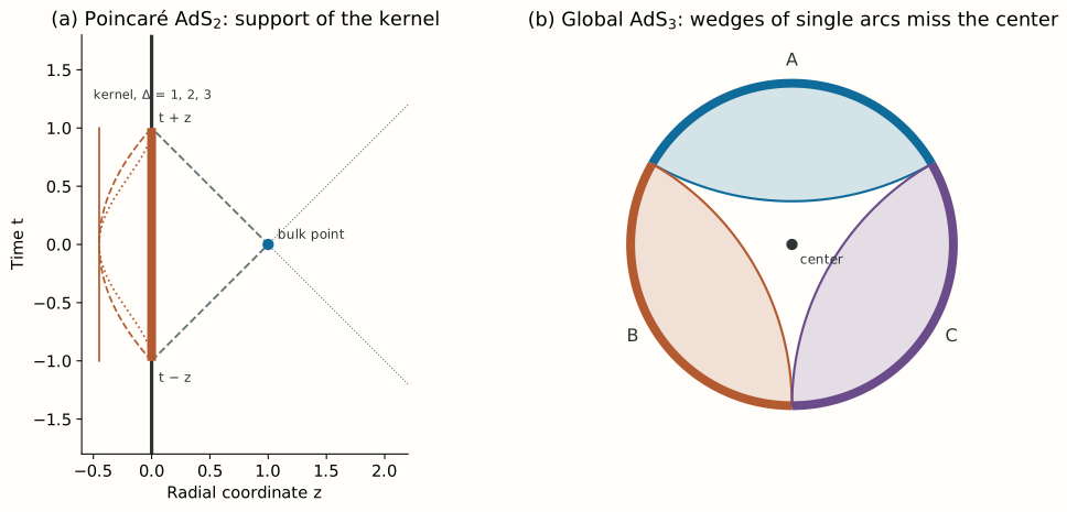
These representatives cannot be the same operator. The representative on $A\cup B$ commutes with every operator on $C$, and the one on $B\cup C$ with every operator on $A$. If they were equal as operators on the whole boundary Hilbert space, the common operator would commute with the algebras of $A$ and of $C$, and under additivity and Haag duality for the boundary theory it would belong to the algebra of $B$. That is impossible: the complementary pair $C\cup A$ also represents the operators at the center, and a noncommuting algebra cannot be represented on the disjoint regions $B$ and $C\cup A$ (Lecture 2, §5.2). Equality with ${\varphi }_{CA}$ as well would make the operator commute with every boundary operator, so that it would be a multiple of the identity. Almheiri, Dong and Harlow resolved the tension by requiring equality only on a code subspace of low-energy bulk states:

$${\varphi }_{AB}V={\varphi }_{BC}V={\varphi }_{CA}V=V{\varphi }_{\mathrm{center}},$$

where $V$ is the isometric encoding of bulk states into boundary states. This is the three-qutrit code of Lecture 2. There, the logical qutrit is recovered from any two shares and from no single share, and the logical operators have different physical representatives on different pairs (Problem 11). [Formal analogy, exact in the three-qutrit code.] Lecture 19 replaces causal wedges by entanglement wedges, Lecture 20 supplies the theorem that turns preserved distinguishability into a decoder, and Lecture 21 derives the relative-entropy identity that makes the code work in holography.

Physical picture: redundancy without cloning. A bulk operator deep in the interior is available from many boundary regions, as a logical qutrit is available from many pairs of shares. Its representatives are different physical operators that act identically on the states the code protects. The redundancy is what protects the bulk against the erasure of any one region, and it is consistent with the no-cloning theorem because the regions overlap. This is an interpretation of the calculation above, made exact in the finite code; in holography it holds within a semiclassical code subspace and to the order at which the bulk effective theory is valid.

7. Self-study: other dimensions and other backgrounds

In AdS${}_{d+1}$ with $d\ge 2$ the kernels are more delicate. In global coordinates Hamilton, Kabat, Lifschytz and Lowe found kernels with real support on the boundary points spacelike separated from the bulk point. In the Poincaré patch the bulk normalizable modes have timelike momenta, ${\omega }^2>|\mathbf{k}{|}^2$, and their construction takes the form

$$\varphi (t,\mathbf{x},z)=c_{\Delta ,d}{\int }_{t^{\prime 2}+|{\mathbf{y}}^{\prime }{|}^2<z^2}d{t}^{\prime }{d}^{d-1}{y}^{\prime }{\left[\frac{z^2-t^{\prime 2}-|{\mathbf{y}}^{\prime }{|}^2}{z}\right]}^{\Delta -d}\mathcal{O}(t+t^{\prime },\mathbf{x}+i{\mathbf{y}}^{\prime }),$$

with the spatial coordinates of the boundary operator continued to imaginary values. For $d=1$ there are no spatial coordinates, and the formula reduces to the kernel of §3. [Stated only — refs: Hamilton–Kabat–Lifschytz–Lowe 2006.] In the AdS–Rindler wedge of a ball, the causal wedge of §2, the same authors again needed a complexified boundary. Morrison later constructed Lorentzian integral kernels for causal wedges, which act on the boundary operators by convolution and apply also to states singular on the Rindler horizon. [Stated only — refs: Morrison 2014.]

In a black-hole background the situation changes. Leichenauer and Rosenhaus showed that in AdS–Schwarzschild the horizon introduces modes with angular momentum much larger than their frequency, trapped behind the centrifugal barrier, whose imprint at the boundary is exponentially small. A kernel that reconstructs them would have to amplify exponentially small data, and no smearing function exists. [Stated only — refs: Leichenauer–Rosenhaus 2013.] The obstruction is absent for global reconstruction in pure AdS. It already appears in the AdS–Rindler wedge of pure AdS, whose horizon admits modes with $|\mathbf{k}|\gg \omega$ that are exponentially suppressed at the boundary, which is why Hamilton, Kabat, Lifschytz and Lowe continued to complexified coordinates there and why Morrison’s Lorentzian construction was needed. It is also one reason why the entanglement-wedge reconstruction of Lectures 19–21 does not proceed by explicit kernels.

8. Self-study: interactions and gravitational dressing

For a weak cubic interaction, the first correction obeys a sourced equation such as

$$(\square -m^2){\varphi }^{(1)}=\lambda {\left({\varphi }^{(0)}\right)}^2,$$

and a Green-function solution adds to the linear smearing an integral of products of boundary operators. Kabat, Lifschytz and Lowe fixed these corrections by requiring that the reconstructed operators commute at bulk spacelike separation, an order-by-order condition in $1/N$ in which large-$N$ factorization is essential. The construction is perturbative, and it requires a prescription for composite operators and boundary conditions.

In gravity a coordinate point is not a diffeomorphism-invariant specification of an observable. One can define relational observables, or dress a field to the boundary by a gravitational Wilson line, and the dressing carries gravitational charge that modifies naive locality statements, as Donnelly and Giddings, and Kabat and Lifschytz, discuss. The phrase “the local bulk algebra” therefore refers to an effective algebra at a stated order in $1/N$ with a chosen dressing. Treating it as an exact tensor factor at finite $N$ would assume what reconstruction is meant to clarify.

9. What to take away

• Exact: the causal wedge of a ball in Poincaré AdS is $|t|+\sqrt{r^2+z^2}<R$, bounded on $t=0$ by the Ryu–Takayanagi hemisphere.
• Exact calculation: in Poincaré AdS${}_2$ a free field of any $\Delta$ is $c_{\Delta }{\int }_{t-z}^{t+z}{\left[(z^2-(t^{\prime }-t{)}^2)/z\right]}^{\Delta -1}\mathcal{O}(t^{\prime })d{t}^{\prime }$, with $c_{\Delta }=\Gamma (\Delta +\frac{1}{2})/(\sqrt{\pi }\Gamma (\Delta ))$, supported on boundary points spacelike separated from the bulk point.
• Exact: the reconstruction is an operator identity in the source-free theory; it does not describe signaling, which is governed by retarded response and bulk microcausality.
• Exact calculation, with a formal analogy: in global AdS${}_3$ the center lies in the wedge of every pair of three equal arcs and of no single arc; its representatives agree on a code subspace, as in the three-qutrit code.
• Stated only: real smearing functions exist in global AdS; in the Poincaré and Rindler charts, kernels of compact support use complexified boundary coordinates, and Morrison’s Lorentzian causal-wedge kernels avoid the continuation; horizons with trapped modes obstruct smearing functions.

10. Looking ahead

Lecture 19 introduces the entanglement wedge, which contains the causal wedge and can be larger, and it computes the change of the entanglement wedge of two intervals when they approach each other. Lecture 20 proves that preserved distinguishability implies an explicit decoder, the Petz map, and Lecture 21 derives, in a sector code and then in holography, the relative-entropy identity on which entanglement-wedge reconstruction rests. Lecture 28 returns to the fixed-background correspondence of Rehren, which relates bulk wedges and boundary double cones as this lecture relates bulk points and boundary intervals.

11. Problem set

Classroom core

1. The causal half-ball. Derive $|t|+\sqrt{r^2+z^2}<R$ from the light cones of the two tips of the boundary diamond.

2. The massless kernel. Differentiate $\frac{1}{2}{\int }_{t-z}^{t+z}\mathcal{O}(u)du$ twice with respect to $t$ and to $z$, and verify the wave equation and the boundary limit.

3. A monochromatic mode. Use Poisson’s integral to evaluate the kernel of §3 on $\mathcal{O}(t)=e^{-i\omega t}$, and check that the result solves the Klein–Gordon equation with $m^2{L}^2=\Delta (\Delta -1)$.

4. The normalization. Show that $c_{\Delta }=\Gamma (\Delta +\frac{1}{2})/(\sqrt{\pi }\Gamma (\Delta ))$ gives $\varphi \to z^{\Delta }\mathcal{O}(t)$, and evaluate $c_{\Delta }$ for $\Delta =1$ and $\Delta =2$.

5. Geodesics of the hyperbolic plane. Show that $\tanh \rho \cos \theta =\cos {\theta }_0$ is a geodesic by writing it as the intersection of the hyperboloid with a plane through the origin, and find its closest approach to the center.

6. Three arcs. Verify that the center of global AdS${}_3$ lies in the wedge of each pair of three equal arcs and of no single arc. What is the smallest single arc whose wedge contains the center?

Self-study consolidation

7. Reconstruction versus response. Can the formula of §3 be read as a boundary source that controls $\varphi (t,z)$ instantaneously?

8. Finite resolution. What is missing when the boundary data are band limited to $|\omega |\le \Lambda$, and what extra assumption would bound the missing part of the bulk field?

9. Depth and resolution. For a bulk point at depth $z$, over what boundary time does the kernel extend? Relate the answer to the relation between depth and resolution of Lecture 15.

10. Why the representatives differ. Show that if ${\varphi }_{AB}={\varphi }_{BC}$ as operators on the boundary Hilbert space, then, under additivity and Haag duality, the common operator belongs to the algebra of $B$.

11. Lecture 2 as a reconstruction. In the code $|j⟩\mapsto 3^{-1/2}{\sum }_k|k⟩|k+j⟩|k+2j⟩$, with arithmetic modulo three, find representatives of the logical $Z$ on shares 1 and 2 and on shares 2 and 3, and show that they differ as operators and agree on the code.

12. Kernels are not unique. In global AdS${}_2$ the normalizable modes have frequencies ${\omega }_n=(\Delta +n)/L$. Show that adding to a kernel any function of boundary time whose Fourier transform vanishes at every $\pm {\omega }_n$ leaves the reconstructed field unchanged.

Research extension

13. The complexified kernel of AdS${}_3$. Evaluate the kernel of §7 for $d=2$ on a normalizable mode $e^{-i\omega t+ikx}z{J}_{\nu }\left(z\sqrt{{\omega }^2-k^2}\right)$ with $\omega >|k|$, and show that it reproduces the mode. Known: Hamilton, Kabat, Lifschytz and Lowe give the general formula; the boundary operator carries only timelike momenta whatever the kernel, and the continuation $x\to x+iy$ is what permits a kernel of compact support. Completion: the mode check with the normalization $c_{\Delta ,2}$, and an explanation of what fails for a kernel with real support.

14. The first interacting correction. For a cubic bulk interaction, construct the correction to the reconstructed field at order $\lambda$ by requiring microcausality with the free field. Known: Kabat, Lifschytz and Lowe show that the correction is a sum over double-trace operators with coefficients fixed by the bulk three-point coupling. Completion: the correction in AdS${}_2$ for one value of $\Delta$, with the region and code subspace on which the expansion is controlled.

15. The obstruction in AdS–Schwarzschild. Estimate, in the WKB approximation, the boundary imprint of a mode with angular momentum $\ell$ and frequency $\omega \ll \ell$ trapped outside the horizon. Known: Leichenauer and Rosenhaus find an imprint exponentially small in $\ell$, which obstructs a smearing function. Completion: the WKB tunneling exponent as a function of $\ell /\omega$ for the BTZ or AdS${}_5$ black hole, and the conclusion for the norm of a would-be kernel.

12. Answer checkpoints

1. A point must lie in the future of $(-R,0,0)$ and in the past of $(R,0,0)$ in the flat half-space: $t+R>\sqrt{r^2+z^2}$ and $R-t>\sqrt{r^2+z^2}$, which together are the stated inequality.

2. ${\partial }_t\varphi =\frac{1}{2}[\mathcal{O}(t+z)-\mathcal{O}(t-z)]$ and ${\partial }_z\varphi =\frac{1}{2}[\mathcal{O}(t+z)+\mathcal{O}(t-z)]$; a second derivative gives ${\partial }_t^2\varphi ={\partial }_z^2\varphi =\frac{1}{2}[{\mathcal{O}}^{\prime }(t+z)-{\mathcal{O}}^{\prime }(t-z)]$. For small $z$, $\varphi =z\mathcal{O}(t)+O(z^3)$.

3. With $\nu =\Delta -\frac{1}{2}$, Poisson’s integral gives $\Gamma (\Delta +\frac{1}{2})(2/\omega {)}^{\nu }{z}^{1/2}{J}_{\nu }(\omega z)e^{-i\omega t}$. The function $f=z^{1/2}{J}_{\nu }(\omega z)$ satisfies $z^2(f^{\prime \prime }+{\omega }^{2}f)=({\nu }^2-\frac{1}{4})f$, and ${\nu }^2-\frac{1}{4}=\Delta (\Delta -1)$.

4. ${\int }_{-1}^1(1-u^2{)}^{\Delta -1}du=\sqrt{\pi }\Gamma (\Delta )/\Gamma (\Delta +\frac{1}{2})$, so $c_{\Delta }$ is its inverse. Then $c_1=\frac{1}{2}$ and $c_2=\Gamma (\frac{5}{2})/\sqrt{\pi }=\frac{3}{4}$.

5. The plane $X_1=X_0\cos {\theta }_0$ through the origin meets the hyperboloid in $\sinh \rho \cos \theta =\cosh \rho \cos {\theta }_0$. It reaches the boundary where $\cos \theta \to \cos {\theta }_0$, and its closest approach is where $|\cos \theta |=1$: at $\theta =0$ with $\tanh {\rho }_{\ast }=\cos {\theta }_0$ when ${\theta }_0<\pi /2$, and at $\theta =\pi$ with $\tanh {\rho }_{\ast }=-\cos {\theta }_0$ when ${\theta }_0>\pi /2$. In both cases $\sinh {\rho }_{\ast }=|\cot {\theta }_0|$.

6. A single arc has ${\theta }_0=\pi /3<\pi /2$, so the geodesic separates it from the center. A pair has ${\theta }_0=2\pi /3>\pi /2$, so its geodesic lies on the far side of the center, which is inside the wedge. A single arc contains the center in its wedge only when it is larger than half the circle; half the circle, ${\theta }_0=\pi /2$, gives a geodesic through the center.

7. No. It is a relation between operators satisfying the source-free equation and the normalizable boundary condition. The response to a boundary source is a different problem, governed by the retarded Green function, whose support is causal.

8. All mode coefficients with $|\omega |>\Lambda$. A bound on the missing bulk contribution requires an assumption on the state, such as an energy bound, since the cutoff alone does not control the high-frequency modes.

9. Over the interval $(t-z,t+z)$, of length $2z$. Deeper points use boundary operators spread over longer times, and a boundary time resolution $\delta t$ limits reconstruction to depths larger than about $\delta t$, as the propagator of Lecture 15 spreads over a region of size of order $z$.

10. The operator commutes with the algebra of $A$, being supported on $B\cup C$, and with the algebra of $C$, being supported on $A\cup B$. By additivity it therefore commutes with the algebra of the arc $A\cup C$, and Haag duality identifies the commutant of that algebra with the algebra of its complement, the arc $B$.

11. Logical $Z$ multiplies $|j⟩$ by ${\zeta }^j$. Since the second share minus the first equals $j$, $Z_1^{†}{Z}_2$ acts on each code term as ${\zeta }^j$; so does $Z_2^{†}{Z}_3$, since the third minus the second also equals $j$. The two operators differ, for instance on the state $|0⟩|1⟩|1⟩$, where the first gives $\zeta$ and the second gives $1$, which lies outside the code.

12. The reconstructed field is a sum over modes, and the kernel enters only through its overlaps with $e^{\mp i{\omega }_{n}t}$. A function whose Fourier transform vanishes at every $\pm {\omega }_n$ has zero overlap with every mode and changes nothing. The boundary operator of global AdS has a discrete spectrum, so many kernels represent the same bulk field.

Wiki connections. subregion–subalgebra duality · holographic dictionary