Lecture 19 — Entanglement wedges and changing reconstruction regions

The causal wedge of Lecture 18 is what a boundary region can reach with signals. The entanglement wedge is what its reduced density matrix can know: the bulk domain of dependence of the region between the boundary region and its Ryu–Takayanagi surface, proposed as the bulk dual of the density matrix by Czech, Karczmarek, Nogueira and Van Raamsdonk, by Wall, and by Headrick, Hubeny, Lawrence and Rangamani. We compute the entanglement wedge of two intervals in the AdS${}_3$ vacuum and follow its transition from two components to one as the intervals approach each other, at the separation where their mutual information switches on. In the connected phase the wedge contains a bridge that no causal curve from either interval can reach, which makes the inclusion of the causal wedge in the entanglement wedge strict. We sketch Wall’s argument for that inclusion, explain why the joint reconstruction of the bridge does not clone bulk information, and compute how far an order-one bulk correction moves the transition.

How to use this lecture

Classroom core, one meeting of three hours. The history (§1, 10 minutes), the definition of the wedge (§2, 20 minutes), and the two intervals and their configurations (§3, 35 minutes) come before a 10-minute break. After it come the mutual information and the cross-ratio (§4, 20 minutes), the bridge that no signal reaches (§5, 25 minutes), and joint access without cloning (§6, 15 minutes), with 45 minutes for Checkpoints 1 and 2 and Problems 4–6; Problems 1–3 complete the core assignment. These allocations are proposals and have not been tested in class.

Self-study. Why the entanglement wedge contains the causal wedge (§7), corrections at a crossing and quantum extremal surfaces (§8), and Problems 7–12, including nesting and the divergence of the mutual information as the intervals touch.

Research extension. The exact four-twist correlator against the minimum of the two candidates, a quantum extremal surface at the crossing, and the holographic proof of strong subadditivity, in Problems 13–15.

Prerequisites. Lecture 2 for secret sharing, Lecture 6 for tensor-network cuts, Lecture 16 for the Ryu–Takayanagi prescription and the interval entropy, Lecture 18 for causal wedges and the three-region example.

What this lecture establishes. The two candidate entropies, the transition at $b/\ell =\sqrt{2}-1$, the homology regions, and the strict inclusion of the causal wedge in the connected entanglement wedge are exact calculations at leading order in $1/c$. The general inclusion theorem is sketched, with the null energy condition as its input. The use of the minimum of two candidates rests on the large-$c$ arguments of Hartman and Faulkner, which are stated with sources. Entanglement-wedge reconstruction itself is stated here; Lecture 20 proves the finite recovery theorem, and Lecture 21 proves the relative-entropy identity in a sector code and sketches the step to reconstruction.

0. Reading

Primary.

• M. Headrick, V. E. Hubeny, A. Lawrence, M. Rangamani, Causality & holographic entanglement entropy (2014).
• A. C. Wall, Maximin Surfaces, and the Strong Subadditivity of the Covariant Holographic Entanglement Entropy (2012).
• X. Dong, D. Harlow, A. C. Wall, Reconstruction of Bulk Operators within the Entanglement Wedge in Gauge-Gravity Duality (2016).

Secondary.

• B. Czech, J. L. Karczmarek, F. Nogueira, M. Van Raamsdonk, The Gravity Dual of a Density Matrix (2012).
• V. E. Hubeny, M. Rangamani, Causal Holographic Information (2012).
• M. Headrick, Entanglement Renyi entropies in holographic theories (2010); T. Hartman, Entanglement Entropy at Large Central Charge (2013); T. Faulkner, The Entanglement Renyi Entropies of Disjoint Intervals in AdS/CFT (2013).

Optional research reading.

• T. Faulkner, A. Lewkowycz, J. Maldacena, Quantum corrections to holographic entanglement entropy (2013), and N. Engelhardt, A. C. Wall, Quantum Extremal Surfaces: Holographic Entanglement Entropy beyond the Classical Regime (2014).
• D. Harlow, TASI Lectures on the Emergence of the Bulk in AdS/CFT (2018), on subregion duality.
• J. Cotler, P. Hayden, G. Penington, G. Salton, B. Swingle, M. Walter, Entanglement Wedge Reconstruction via Universal Recovery Channels (2017).

1. What does a density matrix know?

Lecture 18 reconstructed bulk operators in the causal wedge of a boundary region, the region that the boundary domain can reach with signals and receive signals from. In 2012 Czech, Karczmarek, Nogueira and Van Raamsdonk asked the more basic question of what bulk region the reduced density matrix of a boundary region determines. Their answer, and Wall’s in the same year, pointed beyond the causal wedge to the region bounded by the Ryu–Takayanagi surface. Wall proved, with his maximin construction and the null energy condition, that extremal surfaces lie outside the causal wedge and move away from the boundary as the region grows, and he derived strong subadditivity of the covariant prescription from the same construction. Hubeny and Rangamani proposed at the same time that the area of the rim of the causal wedge measures the information in the region, and they observed that it agrees with the entanglement entropy in the cases where the latter is understood microscopically, such as balls in the vacuum. Headrick, Hubeny, Lawrence and Rangamani named the entanglement wedge in 2014 and proved that the covariant prescription is consistent with boundary causality exactly because the entanglement wedge contains the causal wedge.

The two-interval problem that we work out has its own history. Headrick computed the holographic Rényi entropies of two intervals in 2010, and in 2013 Hartman, in the conformal field theory, and Faulkner, from the saddles of three-dimensional gravity, derived the leading order of the minimum formula. Both rest on the dominance of the vacuum Virasoro block, which Hartman established to all orders in the short-interval expansion for a sparse spectrum of light operators. Dong, Harlow and Wall then proved in 2016 that bulk operators can be reconstructed anywhere in the entanglement wedge, by combining the relative-entropy identity of Lecture 21 with the theory of quantum error correction, and Cotler and collaborators extended it to approximate recovery with the universal recovery channels of Lecture 20.

The question of this lecture is the one the three-qutrit code answered in Lecture 2. Can two observers gain access by pooling their records? Either share of an authorized pair carries no logical state, while the pair recovers it. We will see a geometric version: a union of boundary regions reconstructs a bulk region available to neither component.

2. The region bounded by a surface

For a boundary region $A$ on a static slice, let ${\gamma }_A$ be its Ryu–Takayanagi surface and ${\Sigma }_A$ the bulk spatial region bounded by $A$ and ${\gamma }_A$, as the homology condition of Lecture 16 requires. The entanglement wedge is the bulk domain of dependence

$$E[A]=D_{\mathrm{bulk}}({\Sigma }_A).$$

In a time-dependent state the surface is the extremal surface of Hubeny, Rangamani and Takayanagi and ${\Sigma }_A$ an achronal homology region; with bulk quantum corrections it is the quantum extremal surface of §8. Note that the wedge is a spacetime region, and its observables are the candidates for reconstruction from $A$ within a specified semiclassical code subspace.

For a ball in the vacuum the entanglement wedge is the AdS–Rindler wedge, and it coincides with the causal wedge of Lecture 18: on the slice $t=0$ both are the half-ball bounded by the hemisphere. The difference between the two wedges appears for other regions and other states. The simplest example is two intervals in the vacuum of AdS${}_3$.

3. Two intervals and two configurations

Take two equal intervals on the line,

$$A=[0,\ell ],B=[\ell +b,2\ell +b],b>0.$$

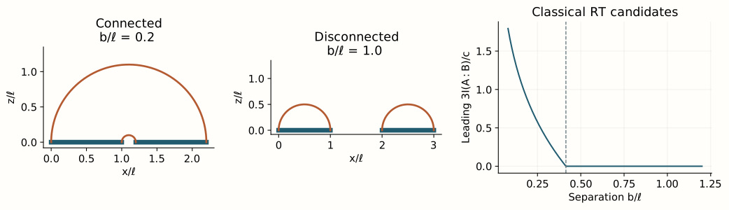
The Ryu–Takayanagi surface of $A\cup B$ is a pair of geodesics joining the four endpoints without crossing, and two pairings compete. In the disconnected configuration each interval is joined to itself. In the connected configuration the outer endpoints $0$ and $2\ell +b$ are joined, and so are the inner endpoints $\ell$ and $\ell +b$. With $S([x_1,x_2])=\frac{c}{3}\log (|x_2-x_1|/ϵ)$ and $c=3L/2G_N$ from Lecture 16,

$$S_{\mathrm{disc}}(A\cup B)=\frac{c}{3}\log \frac{{\ell }^2}{{ϵ}^2},S_{\mathrm{conn}}(A\cup B)=\frac{c}{3}\log \frac{(2\ell +b)b}{{ϵ}^2}.$$

Both configurations satisfy the homology condition, with different regions. In the disconnected configuration ${\Sigma }_{A\cup B}$ is the union of two half-disks of radius $\ell /2$. In the connected one it is the arch between the outer and the inner semicircle, both centered at $x_c=\ell +b/2$,

$${\Sigma }_{\mathrm{conn}}=\left\{{\left(\frac{b}{2}\right)}^2<(x-x_c{)}^2+z^2<{\left(\ell +\frac{b}{2}\right)}^2\right\},$$

which includes a bridge above the gap between the intervals. The prescription selects the smaller entropy. The four endpoint divergences appear in both candidates and cancel in their difference, so the selection is independent of the cutoff. The transition occurs when

$${\ell }^2=b(2\ell +b),\frac{b}{\ell }=\sqrt{2}-1\approx \mathrm{0.414.}$$

For $b/\ell <\sqrt{2}-1$ the connected configuration wins and the wedge of the union is connected. For larger separations it has two components, at this classical order.

Checkpoint 1. Why does the bridge of the connected wedge not belong to the wedge of either interval alone?

Answer. The wedge of $A$ alone is the half-disk of radius $\ell /2$ centered at $\ell /2$, and a point above the gap, at horizontal position $x_c$, is at horizontal distance $(\ell +b)/2>\ell /2$ from its center. The same holds for $B$.

4. Mutual information and the cross-ratio

The mutual information

$$I(A:B)=S(A)+S(B)-S(A\cup B)$$

is finite, as Lecture 8 found on the lattice and Lecture 9 explained with the split property. At leading order in the classical bulk regime,

$$I(A:B)=\frac{c}{3}\max \left\{0,\log \frac{{\ell }^2}{b(2\ell +b)}\right\}.$$

It depends only on the conformal cross-ratio

$$x=\frac{{\ell }^2}{(\ell +b{)}^2},1-x=\frac{b(2\ell +b)}{(\ell +b{)}^2},$$

as $I=\frac{c}{3}\max \{0,\log [x/(1-x)]\}$, with the transition at $x=\frac{1}{2}$. For $b=\ell /4$ the logarithm is $\log (16/9)>0$, and for $b=\ell$ the disconnected configuration wins, which confirms the direction of the transition. As the intervals touch, $b\to 0$, the mutual information diverges as $\frac{c}{3}\log (\ell /2b)$, the holographic counterpart of the lattice divergence of Lecture 8, Problem 14.

The figure shows the selected geodesics on both sides of the transition.

But a vanishing mutual information at order $c$ does not make the boundary state a product. Bulk quantum fields contribute correlations of order one where the order-$c$ term vanishes, and finite-$c$ effects smooth the sharp transition. The minimum of the two candidates is itself a statement about large $c$: Hartman and Faulkner derived it from the dominance of the vacuum conformal block in the four-twist correlator, which requires a sparse spectrum of light operators. [Stated only — refs: Hartman 2013; Faulkner 2013.]

5. The bridge that no signal reaches

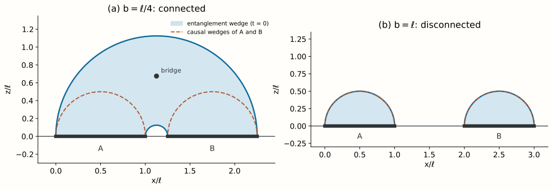
In the connected phase the entanglement wedge of $A\cup B$ is strictly larger than its causal wedge. The causal wedge of the union is the union of the causal wedges of the components,

$$C[A\cup B]=C[A]\cup C[B],$$

because no bulk causal curve connects $D(A)$ with $D(B)$. In the null coordinates $u=t-x$ and $v=t+x$, a future-directed causal curve on the boundary increases both. On $D(A)$ we have $u>-\ell$ and $v<\ell$, and on $D(B)$ we have $u<-(\ell +b)$ and $v>\ell +b$. A curve from $D(A)$ to $D(B)$ would have to decrease $u$, and one from $D(B)$ to $D(A)$ would have to decrease $v$; the obstruction is the gap $b$ between the inner endpoints. In the flat chart of Poincaré AdS${}_3$ bulk causal curves are no faster than boundary ones, since the bulk condition $d{t}^2\ge d{x}^2+d{z}^2$ implies $d{t}^2\ge d{x}^2$, so the same obstruction holds in the bulk. Therefore $J^{+}(D(A))\cap J^{-}(D(B))$ and $J^{+}(D(B))\cap J^{-}(D(A))$ are empty, and only the two separate causal wedges remain. On the slice $t=0$ they are two half-disks of radius $\ell /2$.

The point $(x_c,z)$ above the middle of the gap, with $b/2<z<\ell +b/2$, lies in the arch ${\Sigma }_{\mathrm{conn}}$ and in neither half-disk, by Checkpoint 1. [Exact calculation.] Thus the bridge belongs to the entanglement wedge of the union and to no causal wedge: a boundary observer with access to $A\cup B$ can reconstruct operators there, but cannot reach them with signals, and cannot receive signals from them, within $D(A)\cup D(B)$. The figure compares the two wedges.

Checkpoint 2. In the disconnected phase, are the causal and entanglement wedges of $A\cup B$ equal?

Answer. Yes, at this order. Both are the union of the two half-disks of radius $\ell /2$, since each interval is a ball whose causal and entanglement wedges coincide.

6. Joint access without cloning

For a point in the bridge, neither interval contains an adequate representative of its bulk operators, and the union does. This resembles the authorized pairs of the three-qutrit code, and it extends the three-region example of Lecture 18, §6, where the causal wedges of pairs of arcs already covered the center. The analogy does not identify the geometry with the code. The code provides an exact finite recovery map, while wedge reconstruction uses a semiclassical dictionary within a code subspace and is in general approximate.

Suppose the same noncommuting logical algebra had exact representatives on two disjoint physical factors throughout one code subspace. Operators on disjoint factors commute. The intertwining relation of Lecture 2 would then make every pair of represented logical operators commute on the code, which contradicts the noncommutativity of a full matrix algebra. This is the algebraic no-cloning obstruction. Overlapping boundary regions can represent the same bulk operator because their representatives need not act on disjoint factors. A central, commuting observable can also be available on disjoint regions without cloning anything quantum, as Lecture 5 found for the flux label.

The wedges also respect the order of inclusion. If $A\subset A^{\prime }$, then $E[A]\subset E[A^{\prime }]$: a larger region knows at least as much. For single intervals in the vacuum this is the statement that the semicircle of a subinterval lies inside the half-disk of the interval (Problem 9). Wall proved it for general regions under the null energy condition. [Stated only — refs: Wall 2012.]

Physical picture: knowledge beyond reach. A boundary region can know about bulk events that it cannot influence and cannot hear from within its domain of dependence. The bridge of the connected wedge is the simplest example: its operators are encoded in the correlations between the two intervals, which the mutual information of order $c$ measures; neither interval holds them separately. Reconstruction from quantum correlations and causal access are therefore different notions. This is an interpretation of an exact geometric statement at leading order; its content as a statement about operators is the reconstruction theorem of Dong, Harlow and Wall, whose finite ingredients Lectures 20 and 21 develop.

7. Self-study: why the entanglement wedge contains the causal wedge

The general statement is that the extremal surface of a region lies outside its causal wedge, so that $C[A]\subseteq E[A]$. It holds in bulk spacetimes satisfying the null energy condition, $T_{ab}{k}^a{k}^b\ge 0$ for null $k$. [Sketched — refs: Wall 2012; Headrick–Hubeny–Lawrence–Rangamani 2014.]

The mechanism is focusing. The null geodesics leaving an extremal surface orthogonally start with zero expansion, since extremality is the vanishing of the first variation of area in every normal direction. Along them the Raychaudhuri equation, $d\theta /d\lambda =-{\theta }^2/(d-1)-{\sigma }^2-R_{ab}{k}^a{k}^b$, together with the null energy condition, forces $\theta \le 0$: the congruence can only focus. If the extremal surface were in causal contact with $D(A)$, a null hypersurface through it could be followed to the conformal boundary inside $D(A)$, and near the boundary the expansion of a congruence reaching it is positive, since the area element diverges there. A congruence that starts with zero expansion and can only focus cannot become expanding, so the extremal surface must stay outside the causal wedge. The full argument, which handles caustics and the global structure of the null hypersurfaces with the maximin construction, is in the cited papers.

The inclusion is also what makes the prescription consistent with boundary causality. If the extremal surface of $A$ could be reached from $D(A)$ by a causal curve, a boundary perturbation in $D(A)$ could change the entropy of $A$, which is invariant under unitaries localized in $D(A)$. Headrick, Hubeny, Lawrence and Rangamani turned this observation into their consistency theorem.

8. Self-study: corrections at a crossing

At the next order the entropy is the generalized entropy of Faulkner, Lewkowycz and Maldacena,

$$S(A)=\frac{⟨\mathrm{Area}({\gamma }_A)⟩}{4G_N}+S_{\mathrm{bulk}}({\Sigma }_A)+O(G_N),$$

and Engelhardt and Wall proposed that the surface itself should extremize this combination, the quantum extremal surface. [Stated only — refs: Faulkner–Lewkowycz–Maldacena 2013; Engelhardt–Wall 2014.] Away from a crossing the order-one bulk term cannot change which configuration is selected. Near the crossing the two classical candidates are close, and the bulk term can decide.

The size of the shift follows from the slope of the classical difference. With $y=b/\ell$,

$$S_{\mathrm{disc}}-S_{\mathrm{conn}}=-\frac{c}{3}\log [y(2+y)],{\frac{d}{dy}(S_{\mathrm{disc}}-S_{\mathrm{conn}})|}_{y=\sqrt{2}-1}=-\frac{2\sqrt{2}}{3}c.$$

A bulk entropy difference $\delta S_{\mathrm{bulk}}=S_{\mathrm{bulk}}({\Sigma }_{\mathrm{disc}})-S_{\mathrm{bulk}}({\Sigma }_{\mathrm{conn}})$ between the candidates therefore moves the transition by

$$\delta y\simeq \frac{3\delta S_{\mathrm{bulk}}}{2\sqrt{2}c},$$

a shift of order $1/c$ as long as the slope does not vanish; a positive $\delta S_{\mathrm{bulk}}$ extends the connected phase to larger separations. [Controlled perturbative, in $1/c$.] A large-$c$ expansion can be accurate for each candidate and still fail to select the winner within this window. One should report both candidate values and their difference, and the identity of the selected surface only when the difference is large compared with the corrections.

9. What to take away

• Exact calculation at leading order: two intervals of length $\ell$ at separation $b$ switch from a disconnected to a connected entanglement wedge at $b/\ell =\sqrt{2}-1$, where $I(A:B)=\frac{c}{3}\max \{0,\log [x/(1-x)]\}$ switches on.
• Exact: the causal wedge of the union is the union of the causal wedges, because no causal curve joins the two boundary diamonds; in the connected phase the bridge above the gap lies in the entanglement wedge and in no causal wedge.
• Sketched: under the null energy condition extremal surfaces lie outside the causal wedge, so $C[A]\subseteq E[A]$, and entanglement wedges are nested.
• Exact: joint reconstruction by overlapping regions is consistent with no-cloning, which forbids exact noncommuting representatives on disjoint factors.
• Controlled perturbative: an order-one bulk entropy shifts the transition by $\delta (b/\ell )\simeq 3\delta S_{\mathrm{bulk}}/(2\sqrt{2}c)$.

10. Looking ahead

Lecture 20 turns the statement that distinguishability is preserved into an explicit decoder, the Petz map, and proves the equality theorem that makes this possible. Lecture 21 derives the relative-entropy identity of Jafferis, Lewkowycz, Maldacena and Suh in a sector code and in holography, the identity on which the reconstruction theorem of Dong, Harlow and Wall for the bridge found here rests. Lecture 26 meets the same competition of configurations for a black hole and its radiation, where the connected configuration is an island.

11. Problem set

Classroom core

1. The crossing. Put $y=b/\ell$ and solve $1=y(2+y)$.

2. The cross-ratio. Derive ${\ell }^2/[b(2\ell +b)]=x/(1-x)$.

3. Joint access. For $b=\ell /4$, compute $I(A:B)$ at classical order.

4. The two homology regions. Write the inequalities that define ${\Sigma }_{A\cup B}$ on the slice $t=0$ in both phases, and decide which contains the point $(x_c,\ell /2)$ when $b=\ell /4$.

5. No signal between the diamonds. Show that no causal curve in Poincaré AdS${}_3$ joins $D(A)$ to $D(B)$.

6. The bridge. For $b=\ell /4$, show that $(x_c,z)$ lies in the entanglement wedge of $A\cup B$ and in no causal wedge for $b/2<z<\ell +b/2$.

Self-study consolidation

7. Corrections at a crossing. Let the bulk entropy difference between the candidates be $\delta S_{\mathrm{bulk}}=O(1)$. Estimate the shift of $b/\ell$, and say when the estimate fails.

8. Commuting versus quantum information. Why may a sector label be available on disjoint regions?

9. Nesting. For single intervals $A\subset A^{\prime }$ on the line, show that the semicircle of $A$ lies inside the half-disk of $A^{\prime }$.

10. The rim of the causal wedge. Show that for an interval in Poincaré AdS${}_3$ the rim of the causal wedge, where its future and past boundaries meet, is the Ryu–Takayanagi semicircle, so that the causal holographic information equals the entropy.

11. Subadditivity. Show that the leading-order mutual information is nonnegative in both phases, and identify the inequality that the minimum formula guarantees.

12. Touching intervals. Find the behavior of $I(A:B)$ as $b\to 0$ at fixed $\ell$, and relate it to Lecture 8, Problem 14, and to the split property of Lecture 9.

Research extension

13. The exact correlator. Compare the Rényi entropies from the four-twist correlator of a large-$c$ CFT with the minimum of the two candidates. Known: Hartman shows, to all orders in the short-interval expansion, that the vacuum block dominates when the spectrum of light operators is sparse, and Faulkner obtains the same result from the dominant gravitational saddles; the minimum formula fails for generic finite-$c$ theories. Completion: the statement of the dominance assumption, and the location of the transition obtained from the vacuum block at $n\to 1$.

14. A quantum extremal surface at the crossing. Model the bulk entropy of the bridge by the mutual information of a free bulk field across it, and find the shifted transition. Known: the shift is of order $1/c$ by §8; its sign depends on which configuration has the larger bulk entropy. Completion: the shifted value of $b/\ell$ for one bulk field, with the orders of the neglected terms.

15. Strong subadditivity from geodesics. Prove strong subadditivity for three adjacent intervals in the AdS${}_3$ vacuum by cutting and gluing geodesics. Known: Headrick and Takayanagi gave this argument for the static prescription, and Wall extended it to the covariant one with the maximin construction. Completion: the cut-and-paste inequality with a figure, and the configuration in which it is saturated.

12. Answer checkpoints

1. $y^2+2y-1=0$ gives $y=-1\pm \sqrt{2}$; the positive root is $\sqrt{2}-1$.

2. $(\ell +b{)}^2-{\ell }^2=b(2\ell +b)$, so $1-x=b(2\ell +b)/(\ell +b{)}^2$ and $x/(1-x)={\ell }^2/[b(2\ell +b)]$.

3. ${\ell }^2/[\frac{\ell }{4}(2\ell +\frac{\ell }{4})]=16/9$, so $I=\frac{c}{3}\log \frac{16}{9}$. A positive value alone is not a decoder.

4. Disconnected: $(x-\frac{\ell }{2}{)}^2+z^2<\frac{{\ell }^2}{4}$ or $(x-\frac{3\ell }{2}-b{)}^2+z^2<\frac{{\ell }^2}{4}$. Connected: $\frac{b^2}{4}<(x-x_c{)}^2+z^2<(\ell +\frac{b}{2}{)}^2$. For $b=\ell /4$ the connected phase is selected, since $\frac{1}{4}<\sqrt{2}-1$, and $(x_c,\frac{\ell }{2})$ satisfies $\frac{{\ell }^2}{64}<\frac{{\ell }^2}{4}<\frac{81{\ell }^2}{64}$.

5. A bulk causal curve satisfies $d{t}^2\ge d{x}^2+d{z}^2\ge d{x}^2$, so its projection to the boundary coordinates is causal, and it cannot decrease $u=t-x$ or $v=t+x$ when future directed. Since $u>-\ell$ on $D(A)$ and $u<-(\ell +b)$ on $D(B)$, no such curve runs from $D(A)$ to $D(B)$; since $v<\ell$ on $D(A)$ and $v>\ell +b$ on $D(B)$, none runs back.

6. The point lies in the arch because $b/2<z<\ell +b/2$. Its horizontal distance from the center of either half-disk is $(\ell +b)/2>\ell /2$, so it lies in neither causal wedge.

7. The classical difference has slope $-\frac{2\sqrt{2}}{3}c$ at the crossing, so $\delta y\simeq 3\delta S_{\mathrm{bulk}}/(2\sqrt{2}c)$. The estimate fails when $\delta S_{\mathrm{bulk}}$ is itself of order $c$, or near a point where the slope vanishes.

8. Its algebra is commutative. The no-cloning contradiction requires two noncommuting logical observables, which a classical label does not supply.

9. If $A=[a_1,a_2]\subset A^{\prime }=[a_1^{\prime },a_2^{\prime }]$, a point of the semicircle of $A$ satisfies $(x-\bar{a}{)}^2+z^2=r^2$ with $\bar{a}$ and $r$ its center and radius. Its distance from the center ${\bar{a}}^{\prime }$ of the larger semicircle is at most $|\bar{a}-{\bar{a}}^{\prime }|+r\le r^{\prime }$, because the interval $[\bar{a}-r,\bar{a}+r]$ lies in $[{\bar{a}}^{\prime }-r^{\prime },{\bar{a}}^{\prime }+r^{\prime }]$.

10. The future boundary of the causal wedge is the past light cone of the future tip, $\sqrt{(x-x_0{)}^2+z^2}=R-t$, and the past boundary is the future cone of the past tip, $\sqrt{(x-x_0{)}^2+z^2}=R+t$. They meet at $t=0$ on $(x-x_0{)}^2+z^2=R^2$, the semicircle.

11. In the disconnected phase $I=0$. In the connected phase $I=\frac{c}{3}\log \frac{{\ell }^2}{b(2\ell +b)}>0$, since the connected configuration is selected only when it is smaller. The minimum formula therefore guarantees subadditivity, $S(A\cup B)\le S(A)+S(B)$.

12. $I\simeq \frac{c}{3}\log \frac{\ell }{2b}$, which diverges logarithmically. Touching regions have no split inclusion, and the lattice mutual information of adjacent intervals in Lecture 8 diverges as $a\to 0$; the gap $b$ plays the role of $a$ here, and the holographic formula shows the same logarithmic divergence with the coefficient $c/3$.

Wiki connections. subregion–subalgebra duality · Ryu–Takayanagi formula · quantum extremal surfaces