Lecture 22 — What an entanglement first law implies for gravity

The first law $\delta S=\delta ⟨K⟩$ holds in ordinary quantum mechanics, and by itself it says nothing about gravity. It acquires dynamical content when both sides are identified with bulk quantities, the entropy with an area and the modular energy with the stress tensor read from the metric, and when it is required for every ball. Lashkari, McDermott and Van Raamsdonk, and then Faulkner, Guica, Hartman, Myers and Van Raamsdonk, showed that the requirement is equivalent to the linearized Einstein equations around AdS. We carry out the argument completely for static perturbations of AdS${}_3$. We compute the first-order changes of the geodesic length and of the modular energy, construct the one-form whose exterior derivative is the linearized Hamiltonian constraint weighted by the Killing vector of the AdS–Rindler wedge, and prove the elementary injectivity that turns the first law for all intervals into the vanishing of the constraint. The general statement, in any dimension and with the Iyer–Wald form, is then stated with the steps that the three-dimensional case makes visible.

How to use this lecture

Classroom core, one meeting of three hours. The history (§1, 10 minutes), the boundary side (§2, 15 minutes), the area variation at an extremal surface (§3, 20 minutes), and the AdS–Rindler Killing vector (§4, 15 minutes) come before a 10-minute break. After it come the first law as an integral identity in AdS${}_3$ (§5, 40 minutes), injectivity (§6, 25 minutes), and the extension to all frames (§7, 15 minutes), with 30 minutes for Checkpoints 1 and 2 and Problems 4–6; Problems 1–3 complete the core assignment. These allocations are proposals and have not been tested in class.

Self-study. The Iyer–Wald construction in general (§8), the thermal family as a check (§9), the scope of the conclusion (§10), and Problems 7–12, including the static vacuum solutions and the recursion behind injectivity.

Research extension. Higher-curvature theories, the other components from boosted frames, and the second order through canonical energy, in Problems 13–15.

Prerequisites. Lecture 11 for the modular Hamiltonian of a ball and the first law, Lecture 13 for Poincaré AdS, Lecture 15 for the scalar near-boundary expansion and one-point functions, whose metric counterpart §2 states, Lecture 16 for the Ryu–Takayanagi geodesics and $c=3L/2G_N$, Lecture 21 for the stationarity of the area at an extremal surface. First variations of actions and Stokes’ theorem.

What this lecture establishes. For static perturbations of Poincaré AdS${}_3$ in Fefferman–Graham gauge, the linearized field equations, the first-order changes of entropy and modular energy, the integral identity relating their difference to the Hamiltonian constraint, and the injectivity of the resulting transform for perturbations analytic in the radial coordinate are exact calculations, checked symbolically. The use of all Lorentz frames to reach every component, the covariant phase-space construction of Iyer and Wald, and the theorem of Faulkner, Guica, Hartman, Myers and Van Raamsdonk in general dimension are stated with sources.

0. Reading

Primary.

• N. Lashkari, M. B. McDermott, M. Van Raamsdonk, Gravitational Dynamics From Entanglement “Thermodynamics” (2013).
• T. Faulkner, M. Guica, T. Hartman, R. C. Myers, M. Van Raamsdonk, Gravitation from Entanglement in Holographic CFTs (2014).
• V. Iyer, R. M. Wald, Some Properties of Noether Charge and a Proposal for Dynamical Black Hole Entropy (1994).

Secondary.

• R. M. Wald, Black Hole Entropy is Noether Charge (1993).
• D. D. Blanco, H. Casini, L.-Y. Hung, R. C. Myers, Relative Entropy and Holography (2013).
• S. de Haro, K. Skenderis, S. N. Solodukhin, Holographic Reconstruction of Spacetime and Renormalization in the AdS/CFT Correspondence (2000), for the holographic stress tensor.

Optional research reading.

• T. Jacobson, Thermodynamics of Spacetime: The Einstein Equation of State (1995), and Entanglement Equilibrium and the Einstein Equation (2015).
• B. Swingle, M. Van Raamsdonk, Universality of Gravity from Entanglement (2014).
• T. Faulkner, F. M. Haehl, E. Hijano, O. Parrikar, C. Rabideau, M. Van Raamsdonk, Nonlinear Gravity from Entanglement in Conformal Field Theories (2017), and N. Lashkari, M. Van Raamsdonk, Canonical Energy is Quantum Fisher Information (2015).

1. Where does dynamics enter an entropy identity?

In 1995 Jacobson derived Einstein’s equations from thermodynamics. He required that the Clausius relation $\delta Q=T\delta S$ hold for every local Rindler horizon, with the entropy proportional to the area and the temperature equal to the Unruh temperature of Lecture 10, and found that the equation of state of spacetime is Einstein’s equation. The holographic version of the idea came from the first law of entanglement. Bhattacharya, Nozaki, Takayanagi and Ugajin found the law for small holographic excitations in 2012, and Blanco, Casini, Hung and Myers explained it in 2013 as the first-order vanishing of relative entropy, as Lecture 11 showed. Later in 2013 Lashkari, McDermott and Van Raamsdonk inverted the logic. They assumed the Ryu–Takayanagi formula and the holographic stress tensor, required the first law for every ball, and derived Einstein’s equations at linear order around AdS.

Faulkner, Guica, Hartman, Myers and Van Raamsdonk then gave a covariant proof in every dimension, based on the Noether charge of Wald and the covariant phase space of Iyer and Wald. The first law for all balls is exactly equivalent to the linearized gravitational equations; for Wald entropy functionals it gives the linearized equations of the corresponding higher-curvature theory, and the same method derives the holographic stress tensor from the entropy formula. Swingle and Van Raamsdonk showed that the leading $1/N$ correction to the first law supplies the bulk stress tensor as the source of the linearized equations, and in 2017 Faulkner and collaborators showed, for states prepared by sources in the Euclidean path integral, that the geometry representing the entanglement entropies of balls satisfies Einstein’s equations up to second order.

This lecture makes the logical structure explicit in the one case where every step can be written on the page, static perturbations of AdS${}_3$. The first law is a quantum identity. The dynamical content comes from the two dictionary entries and from the family of regions.

2. The boundary side

For a ball $B$ of radius $R$ in the vacuum of a conformal field theory, Lecture 11 found

$$\delta ⟨K_B⟩=2\pi {\int }_B{d}^{d-1}x\frac{R^2-r^2}{2R}\delta ⟨T_{00}⟩,$$

and the first law equates it to $\delta S_B$ for every differentiable family of states. No bulk equation has been assumed.

Suppose now that the theory has a semiclassical Einstein dual. Two dictionary entries are needed. The entropy is the area of the Ryu–Takayanagi surface, $\delta S_B=\delta A({\gamma }_B)/4G_N$ at leading order. The stress tensor is read from the metric in Fefferman–Graham gauge,

$$d{s}^2=\frac{L^2}{z^2}\left(d{z}^2+g_{\mu \nu }(x,z)d{x}^{\mu }d{x}^{\nu }\right),g_{\mu \nu }={\eta }_{\mu \nu }+z^d{g}_{\mu \nu }^{(d)}(x)+\cdots ,$$

as $⟨T_{\mu \nu }⟩=\frac{d{L}^{d-1}}{16\pi G_N}{g}_{\mu \nu }^{(d)}$ for a flat boundary without sources, the metric counterpart of the scalar response of Lecture 15. [Stated only — refs: de Haro–Skenderis–Solodukhin 2000.] In $d=2$ this is $⟨T_{\mu \nu }⟩=\frac{L}{8\pi G_N}{g}_{\mu \nu }^{(2)}=\frac{c}{12\pi }{g}_{\mu \nu }^{(2)}$. These two entries are the essential inputs beyond the first law.

3. The area varies only through the metric

Let $g_{ab}\to g_{ab}+h_{ab}$, and let $e_i^a$ be the tangent vectors of the unperturbed extremal surface, with induced metric ${\gamma }_{ij}$. The first-order change of the area due to $h$ is

$$\delta A=\frac{1}{2}{\int }_{{\gamma }_B}\sqrt{\gamma }{\gamma }^{ij}{h}_{ab}{e}_i^a{e}_j^b.$$

The surface also moves, but its displacement does not contribute at first order, because the unperturbed surface is extremal, with fixed anchoring at the boundary and a consistent regulator. This is the functional version of a familiar fact: for a stationary function $f(x,\lambda )$ the first derivative of $f(x(\lambda ),\lambda )$ is ${\partial }_{\lambda }f$, since ${\partial }_{x}f=0$ at the stationary point (Problem 1). The displacement matters at second order, and near degeneracies a naive expansion may fail.

For the semicircle $x-x_0=R\cos \theta$, $z=R\sin \theta$ of Poincaré AdS${}_3$ and a perturbation $g_{xx}=1+H_{xx}$ on the slice $t=0$, the line element is $\frac{L}{z}\sqrt{d{z}^2+(1+H_{xx})d{x}^2}$. Along the semicircle $d{x}^2/(d{x}^2+d{z}^2)={\sin }^2\theta$ and $z=R\sin \theta$, so

$$\delta S_B=\frac{L}{8G_N}{\int }_0^{\pi }d\theta \sin \theta H_{xx}(x_0+R\cos \theta ,R\sin \theta ).$$

4. The AdS–Rindler Killing vector

For the ball of radius $R$ centered at the origin of the Poincaré patch of AdS${}_{d+1}$,

$${\xi }_B=\frac{\pi }{R}\left[\left(R^2-z^2-t^2-r^2\right){\partial }_t-2t\left(z{\partial }_z+x^i{\partial }_i\right)\right]$$

is a Killing vector of the bulk metric; the course scripts verify the Killing equation in AdS${}_4$. At $z=0$ it reduces to the modular vector $\zeta$ of Lecture 11. At $t=0$ it vanishes on the hemisphere $z^2+r^2=R^2$, the Ryu–Takayanagi surface, which is therefore the bifurcation surface of a Killing horizon: the boundary of the AdS–Rindler wedge, the entanglement wedge of the ball. On the slice $t=0$ the vector is ${\xi }_B={\xi }^t{\partial }_t$ with

$${\xi }^t=\frac{\pi }{R}\left(R^2-z^2-r^2\right),$$

positive inside the wedge. The bulk modular flow is the flow of ${\xi }_B$, and the figure shows it.

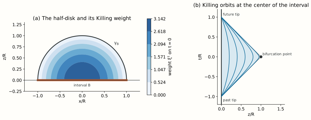
This geometry is why a first law for black holes can be applied although the background is pure AdS. The horizon is the Killing horizon of the AdS–Rindler flow of the region, and the entanglement entropy of the ball is the entropy of that horizon, as Lecture 16, §7, showed through the map of Casini, Huerta and Myers.

5. Static AdS${}_3$: the first law as an integral identity

Consider static perturbations of Poincaré AdS${}_3$ in Fefferman–Graham gauge,

$$d{s}^2=\frac{L^2}{z^2}\left[d{z}^2-(1-H_{tt}(x,z))d{t}^2+(1+H_{xx}(x,z))d{x}^2\right],$$

with $H_{tt}$ and $H_{xx}$ small and of order $z^2$ at the boundary, $H=z^2(\cdots )+O(z^3)$. The linearized Einstein operator $\delta E_{ab}=\delta (G_{ab}+\Lambda g_{ab})$, with $\Lambda =-1/L^2$, has the components

$$\delta E_{tt}=-\frac{z}{2}{\partial }_z\left(\frac{{\partial }_z{H}_{xx}}{z}\right),\delta E_{xx}=-\frac{z}{2}{\partial }_z\left(\frac{{\partial }_z{H}_{tt}}{z}\right),$$ $$\delta E_{zz}=\frac{{\partial }_z{H}_{tt}-{\partial }_z{H}_{xx}}{2z}-\frac{1}{2}{\partial }_x^2{H}_{tt},\delta E_{xz}=\frac{1}{2}{\partial }_x{\partial }_z{H}_{tt}.$$

[Exact calculation, checked symbolically.] The component $\delta E_{tt}$ is the Hamiltonian constraint on the slices $t=\text{constant}$. Its vanishing, with the boundary condition, gives $H_{xx}=z^{2}b(x)$, and the other equations then force $H_{tt}=z^{2}e$ with $e=b$ constant (Problem 9). A static state of a two-dimensional conformal field theory on a line has constant energy density, by conservation and tracelessness of the stress tensor, and the static solutions are the small-temperature expansion of the BTZ black hole of §9.

For an interval of radius $R$ centered at $x_0$, the entropy change is the integral of §3. For the modular energy we use the traceless form of the stress tensor, $⟨T_{tt}⟩=⟨T_{xx}⟩=\frac{L}{8\pi G_N}b(x)$, where $b$ is the coefficient of $z^2$ in $H_{xx}$; the equality of the two components is the boundary limit of the equation $\delta E_{zz}=0$. Then

$$\delta ⟨K_B⟩=\frac{L}{8G_{N}R}{\int }_{x_0-R}^{x_0+R}dx(R^2-(x-x_0{)}^2)b(x).$$

Both sides are functionals of $H_{xx}$ alone, and their difference can be computed exactly. Consider on the half-disk $\Sigma =\{(x-x_0{)}^2+z^2<R^2\}$ of the slice $t=0$ the one-form

$$\chi =\frac{L}{16G_{N}R}\left[(R^2-(x-x_0{)}^2-z^2)\frac{{\partial }_z{H}_{xx}}{z}+2H_{xx}\right]dx.$$

On the semicircle the first term vanishes and $\chi =\frac{L}{8G_{N}R}{H}_{xx}dx$. At the boundary, $H_{xx}=z^{2}b+O(z^3)$ gives ${\partial }_z{H}_{xx}/z\to 2b$, and $\chi \to \frac{L}{8G_{N}R}(R^2-(x-x_0{)}^2)bdx$. Its exterior derivative is

$$d\chi =-{\partial }_z{\chi }_{x}dx\wedge dz=\frac{L}{8\pi G_N}\frac{{\xi }^t}{z}\delta E_{tt}dx\wedge dz,$$

since ${\partial }_z$ of the bracket is $(R^2-(x-x_0{)}^2-z^2){\partial }_z({\partial }_z{H}_{xx}/z)$, the terms from differentiating the weight and from $2H_{xx}$ cancelling. Stokes’ theorem on $\Sigma$, with the boundary traversed along $z=0$ from $x_0-R$ to $x_0+R$ and back along the semicircle, where $dx=-R\sin \theta d\theta$, gives the boundary term $\delta ⟨K_B⟩$ and the arc term $-\delta S_B$. Therefore

$$\delta ⟨K_B⟩-\delta S_B=\frac{L}{8\pi G_N}{\int }_{\Sigma }dxdz\frac{{\xi }^t}{z}\delta E_{tt}.$$

[Exact calculation, checked symbolically and numerically for perturbations that violate the field equations.] The difference between modular energy and entropy is the Hamiltonian constraint integrated over the entanglement wedge with the weight of the Killing vector, and the first law for the interval is the vanishing of that weighted integral.

Checkpoint 1. Why does the one-form contain the derivative ${\partial }_z{H}_{xx}$, although neither $\delta S_B$ nor $\delta ⟨K_B⟩$ does?

Answer. The weight $R^2-(x-x_0{)}^2-z^2$ multiplying it vanishes on the semicircle and reduces to the modular weight at the boundary, where ${\partial }_z{H}_{xx}/z\to 2b$. The derivative is needed in the interior, so that the exterior derivative reproduces the constraint, and it is invisible on the two boundaries.

6. From all intervals to the constraint

One interval is not enough. A function can integrate to zero over one region without vanishing, as $f(x)=x$ does on $[-1,1]$ (Problem 3). The first law holds for every interval, and the family of half-disks is rich enough to recover the integrand.

Claim (injectivity). Proved, for perturbations analytic in $z$. Let $F=\delta E_{tt}/z$, and suppose $F(x,z)={\sum }_n{z}^n{f}_n(x)$ is real analytic in $z\ge 0$, with Fourier-transformable coefficients such that ${\sum }_n{r}^n\Vert {\hat{f}}_n{\Vert }_{L^1}<\infty$ for some $r>0$. If ${\int }_{\Sigma }{\xi }^{t}Fdxdz=0$ for every center $x_0$ and radius $R$, then $F=0$.

Proof. Write $I(x_0,R)={\int }_{\Sigma }(R^2-(x-x_0{)}^2-z^2)Fdxdz$. The weight vanishes on the boundary of $\Sigma$, so differentiating with respect to $R$ gives ${\partial }_{R}I=2R{\int }_{\Sigma }F$. The vanishing of $I$ for all $R$ therefore makes ${\int }_{\Sigma }F$ vanish for all $R$, and a second derivative gives the semicircle means,

$${\int }_0^{\pi }d\theta F(x_0+R\cos \theta ,R\sin \theta )=0\text{for all }{x}_0,R.$$

In Fourier space in $x_0$, with ${\hat{f}}_n(k)$ the transforms of the coefficients,

$$\sum _n{\hat{f}}_n(k)R^n{\mathcal{J}}_n(kR)=0,{\mathcal{J}}_n(u)={\int }_0^{\pi }d\theta e^{iu\cos \theta }{\sin }^n\theta =\sum _{j\ge 0}{c}_{n,j}{u}^{2j},$$

with $c_{n,0}={\int }_0^{\pi }{\sin }^n\theta d\theta >0$. The coefficient of $R^m$ is ${\sum }_j{\hat{f}}_{m-2j}(k)c_{m-2j,j}{k}^{2j}$, a triangular system with nonzero diagonal: the coefficient of $R^0$ gives ${\hat{f}}_0=0$, that of $R^1$ gives ${\hat{f}}_1=0$, and each later one gives ${\hat{f}}_m=0$ once the lower coefficients vanish. Therefore $F$ vanishes for $z<r$, where the series converges and the exchanges of sums, integrals and Fourier transforms are justified, and by analyticity everywhere. $\square$

The first law for all intervals on the slice $t=0$ is thus equivalent to $\delta E_{tt}=0$ everywhere, and with the boundary condition to $H_{xx}=z^{2}b(x)$: the linearized Hamiltonian constraint. [Exact.] The injectivity step, which in general dimension is a statement about integral transforms over hemispheres, is elementary here. The analyticity hypothesis can be weakened, but some regularity and decay are needed, and the argument uses them.

Checkpoint 2. Which step of the argument used that the first law holds for intervals of every size, and which used every position?

Answer. The two derivatives with respect to $R$ used every size, and the Fourier transform in $x_0$ used every position. Neither alone suffices.

7. All frames and all components

Note that the slice $t=0$ constrains only the component $\delta E_{tt}$, and it leaves $H_{tt}$ free. The other constraints come from intervals on the slices of boosted frames, where the modular energy involves $⟨T_{tx}⟩$ and $⟨T_{xx}⟩$ and the entropy the corresponding components of the metric. On the slice of a frame with unit timelike vector $u$, the same argument gives $u^a{u}^b\delta E_{ab}=0$, and requiring it for every boost makes all components $\delta E_{\mu \nu }$ with boundary indices vanish; in two dimensions ${\cosh }^2\eta \delta E_{tt}+2\cosh \eta \sinh \eta \delta E_{tx}+{\sinh }^2\eta \delta E_{xx}=0$ for all $\eta$ forces each term to vanish. The components $\delta E_{z\mu }$ and $\delta E_{zz}$ then follow from the Bianchi identity with the boundary conditions. [Stated only — refs: Faulkner–Guica–Hartman–Myers–Van Raamsdonk 2014.] In general dimension the conclusion is

$$\delta \left(G_{ab}+\Lambda g_{ab}\right)=0$$

for the classical vacuum perturbation problem, and conversely every solution satisfies the first law for all balls.

With bulk quantum matter the entropy is the generalized entropy of Lecture 21, and its first law supplies the bulk modular energy; together with the perturbative dictionary this gives the corresponding sourced equations. The order counting matters: the stress tensor of a scalar with zero background value is quadratic in its amplitude, so it sources the metric at second order (Problem 8).

8. Self-study: the Iyer–Wald construction

The one-form of §5 is a special case of a general construction. For a covariant Lagrangian $\mathbf{L}[g]$, the variation $\delta \mathbf{L}=\mathbf{E}\delta g+d\mathbf{\theta }(\delta g)$ defines the field equations $\mathbf{E}$ and the symplectic potential $\mathbf{\theta }$. For a vector field $\xi$, the Noether current ${\mathbf{J}}_{\xi }=\mathbf{\theta }({\mathcal{L}}_{\xi }g)-\xi \cdot \mathbf{L}$ can be written as $d{\mathbf{Q}}_{\xi }$ plus a combination of the constraints, where ${\mathbf{Q}}_{\xi }$ is the Noether charge. Varying this relation gives the fundamental identity

$$\mathbf{\omega }(g;\delta g,{\mathcal{L}}_{\xi }g)=d[\delta {\mathbf{Q}}_{\xi }-\xi \cdot \mathbf{\theta }(\delta g)]+{\xi }^a\delta {\mathbf{C}}_a,$$

where $\mathbf{\omega }$ is the symplectic current and $\delta {\mathbf{C}}_a$ are the linearized constraints. For a Killing vector of the background, ${\mathcal{L}}_{\xi }g=0$ and $\mathbf{\omega }$ vanishes, so the form $\mathbf{\chi }=\delta {\mathbf{Q}}_{\xi }-\xi \cdot \mathbf{\theta }(\delta g)$ satisfies $d\mathbf{\chi }=-{\xi }^a\delta {\mathbf{C}}_a$. [Sketched — refs: Iyer–Wald 1994; Wald 1993.] For Einstein gravity ${\mathbf{Q}}_{\xi }=-\frac{1}{16\pi G_N}{\mathbf{ϵ}}_{ab}{\nabla }^a{\xi }^b$. Wald’s result that the Noether charge on the bifurcation surface of a Killing horizon is the entropy gives ${\int }_{{\gamma }_B}\mathbf{\chi }\propto \delta A/4G_N$, and the asymptotic falloff gives ${\int }_B\mathbf{\chi }\propto \delta ⟨K_B⟩$. Stokes’ theorem is then the integral identity of §5, in any dimension and for any Lagrangian with its Wald entropy. [Stated only — refs: Faulkner–Guica–Hartman–Myers–Van Raamsdonk 2014.]

9. Self-study: the thermal family as a check

For a two-dimensional conformal field theory at small temperature, Lecture 11 found

$$\delta S_{(-R,R)}=\frac{2c{\pi }^2{R}^2}{9}\delta (T^2)=\delta ⟨K_B⟩.$$

The same numbers follow from §5. The BTZ black hole at small temperature is the static solution $H_{xx}=H_{tt}=z^{2}b$ with $\frac{L}{8\pi G_N}b=\frac{\pi c}{6}{T}^2$, that is, $b=2{\pi }^2{T}^2$. The integral of §3 gives $\delta S=\frac{L}{8G_N}{R}^{2}b{\int }_0^{\pi }{\sin }^3\theta d\theta =\frac{L}{6G_N}{R}^{2}b$, which with $c=3L/2G_N$ is $\frac{2c{\pi }^2{R}^2{T}^2}{9}$. The exact thermal entropy of the interval, $\frac{c}{3}\log [\frac{\beta }{\pi ϵ}\sinh \frac{2\pi R}{\beta }]$, reproduced by the BTZ geodesic in Lecture 16, agrees with this at order $T^2$. This checks a known solution and the dictionary; the proof that every perturbation satisfies the field equations is the content of §§5–7.

10. The scope of “gravity from entanglement”

The conclusion is conditional and linearized. It constrains a bulk description that is already equipped with a geometric entropy functional and a stress-tensor dictionary, and it does not show that an arbitrary quantum system has an Einstein spacetime, nor that the first law alone fixes nonlinear dynamics. At second order the relative entropy of a ball, which the first law sets to zero at first order, becomes the canonical energy of the perturbation in the AdS–Rindler wedge, and Faulkner and collaborators showed that the entropies of balls still have a geometric representation that satisfies Einstein’s equations to second order. [Stated only — refs: Lashkari–Van Raamsdonk 2015; Faulkner et al. 2017.]

Changing the gravitational action changes the entropy functional and the resulting linearized equations. This dependence is informative: the geometric dictionary carries dynamical content, and the first law transfers it from entropy to the metric.

11. What to take away

• Exact: the area of an extremal surface varies at first order only through the metric, and the AdS–Rindler Killing vector of a ball vanishes on its Ryu–Takayanagi surface and reduces at the boundary to the modular vector of Lecture 11.
• Exact calculation: for static perturbations of AdS${}_3$, $\delta ⟨K_B⟩-\delta S_B=\frac{L}{8\pi G_N}{\int }_{\Sigma }\frac{{\xi }^t}{z}\delta E_{tt}$, obtained by Stokes’ theorem from an explicit one-form.
• Proved, under analyticity: the vanishing of this integral for all intervals implies $\delta E_{tt}=0$, by two radial derivatives and a triangular recursion; the first law for all intervals on a slice is the linearized Hamiltonian constraint.
• Stated only: all Lorentz frames give all constraints and, with the Bianchi identity, the linearized Einstein equations in every dimension; the Iyer–Wald form is the general version of the one-form, and Wald entropy functionals give the linearized equations of higher-curvature theories.

12. Looking ahead

Lecture 23 turns to thermal states and black holes, where the entropy of the horizon is the Bekenstein–Hawking entropy and the thermal family of §9 is the small-temperature end of the BTZ geometry. Lectures 25–27 use the generalized entropy whose first law was mentioned in §7, and Lecture 31 asks what replaces the Killing flow of §4 when no symmetry is available.

13. Problem set

Classroom core

1. The surface displacement. For a stationary function $f(x,\lambda )$, show why $x^{\prime }(0)$ drops out of the first derivative of $f(x(\lambda ),\lambda )$.

2. The Killing vector. Evaluate ${\xi }_B$ on $t=0$, $z^2+r^2=R^2$, and at $z=0$.

3. One integral versus all integrals. Give a nonzero function with zero integral on $[-1,1]$, and explain why the family of balls is essential.

4. The length variation. Derive $\delta S_B=\frac{L}{8G_N}{\int }_0^{\pi }\sin \theta H_{xx}d\theta$ from the line element on the slice $t=0$.

5. The boundary values of the one-form. Verify the values of $\chi$ on the semicircle and at $z\to 0$ for $H_{xx}=z^{2}b(x)+z^3\beta (x)$.

6. The exterior derivative. Compute $-{\partial }_z{\chi }_x$ and show that it equals $\frac{L}{8\pi G_N}\frac{{\xi }^t}{z}\delta E_{tt}$ with $\delta E_{tt}=-\frac{z}{2}{\partial }_z(z^{-1}{\partial }_z{H}_{xx})$.

Self-study consolidation

7. The gravitational inputs. List the steps of the argument that go beyond the first law of entanglement.

8. Perturbative order. Why might a scalar perturbation not source the metric at first order in its amplitude?

9. Static solutions. From the four linearized equations of §5, show that the static vacuum perturbations vanishing at the boundary are $H_{tt}=H_{xx}=e{z}^2$ with $e$ constant, and relate $e$ to the temperature of a BTZ black hole.

10. Two radial derivatives. Show that the vanishing of ${\int }_{\Sigma }{\xi }^{t}F$ for all $R$ implies the vanishing of the semicircle means of $F=\delta E_{tt}/z$.

11. The triangular recursion. Compute $c_{n,0}$ for $n=0,1,2$ and $c_{0,1}$, and carry out the recursion of §6 to order $R^2$.

12. The thermal family. Expand $\frac{c}{3}\log \frac{\sinh x}{x}$ with $x=2\pi RT$ and check the first law of §9 at order $T^2$.

Research extension

13. Higher-curvature gravity. Replace the area by the Wald entropy of a higher-curvature action and rederive the identity of §5. Known: Faulkner, Guica, Hartman, Myers and Van Raamsdonk obtain the linearized equations of the corresponding theory; keeping the area while changing the equations is inconsistent. Completion: the modified one-form and constraint for one example, such as a Gauss–Bonnet term in higher dimension.

14. Boosted frames. Repeat the construction of §5 for intervals on the slices of a boosted frame, and show that the first law for all of them gives $\delta E_{tx}=0$ and constrains $H_{tt}$. Known: the full set of constraints follows from all frames, and the remaining equations from the Bianchi identity. Completion: the one-form for a boosted interval, and the demonstration that $H_{tt}=z^{3}f(x)$ violates the first law on some boosted interval.

15. Second order. Show that the relative entropy of a ball between a perturbed state and the vacuum equals, at quadratic order, the canonical energy of the metric perturbation in the AdS–Rindler wedge. Known: Lashkari and Van Raamsdonk prove the equality of quantum Fisher information and canonical energy, and Faulkner and collaborators derive the second-order equations from it. Completion: the argument for static perturbations of AdS${}_3$ with the one-form of §5, and a check of positivity for one perturbation.

14. Answer checkpoints

1. The chain rule gives ${\partial }_{\lambda }f+{\partial }_{x}f{x}^{\prime }(0)$, and ${\partial }_{x}f=0$ at the stationary point. The area argument is its functional version, with the embedding of the surface in the role of $x$.

2. On $t=0$ and $z^2+r^2=R^2$ the time component is proportional to $R^2-z^2-r^2=0$, and the others are proportional to $t=0$. At $z=0$ the vector becomes $\frac{\pi }{R}[(R^2-t^2-r^2){\partial }_t-2t{x}^i{\partial }_i]$, the modular vector $\zeta$ of Lecture 11.

3. $f(x)=x$. A single integral cannot detect an integrand of changing sign, and only the whole family of intervals, varied in size and position, determines the integrand.

4. The length element is $\frac{L}{z}\sqrt{d{z}^2+(1+H_{xx})d{x}^2}=\frac{L}{z}\sqrt{d{x}^2+d{z}^2}(1+\frac{1}{2}{H}_{xx}\frac{d{x}^2}{d{x}^2+d{z}^2})$ at first order. On the semicircle $\sqrt{d{x}^2+d{z}^2}=Rd\theta$, $z=R\sin \theta$ and $d{x}^2/(d{x}^2+d{z}^2)={\sin }^2\theta$, so $\delta (\text{length})=\frac{L}{2}{\int }_0^{\pi }\sin \theta H_{xx}d\theta$, and $\delta S=\delta (\text{length})/4G_N$.

5. On the semicircle the weight vanishes, leaving $\frac{L}{16G_{N}R}\cdot 2H_{xx}$. At the boundary ${\partial }_z{H}_{xx}/z=2b+3\beta z\to 2b$ and $2H_{xx}\to 0$, leaving $\frac{L}{16G_{N}R}(R^2-(x-x_0{)}^2)2b$.

6. With $w=R^2-(x-x_0{)}^2-z^2$, ${\partial }_z[w{\partial }_{z}H/z+2H]=-2z{\partial }_{z}H/z+w{\partial }_z({\partial }_{z}H/z)+2{\partial }_{z}H=w{\partial }_z({\partial }_{z}H/z)$. Thus $-{\partial }_z{\chi }_x=-\frac{L}{16G_{N}R}w{\partial }_z({\partial }_{z}H/z)$, and with ${\xi }^t=\frac{\pi }{R}w$ and $\delta E_{tt}=-\frac{z}{2}{\partial }_z({\partial }_{z}H/z)$ this is $\frac{L}{8\pi G_N}\frac{{\xi }^t}{z}\delta E_{tt}$.

7. The geometric entropy functional, the stress-tensor dictionary, the covariant phase-space identity, and the injectivity and constraint-propagation arguments.

8. Around $\varphi =0$ the stress tensor is quadratic in $\varphi$ and its derivatives, so the metric correction it sources is of second order in the amplitude.

9. $\delta E_{tt}=0$ with $H_{xx}\to 0$ gives $H_{xx}=z^{2}b(x)$, and $\delta E_{xx}=0$ gives $H_{tt}=z^{2}e(x)$. Then $\delta E_{xz}=z{e}^{\prime }(x)=0$ makes $e$ constant, and $\delta E_{zz}=e-b-\frac{1}{2}{z}^2{e}^{\prime \prime }=0$ gives $b=e$. With $\frac{L}{8\pi G_N}e=\frac{\pi c}{6}{T}^2$ and $c=3L/2G_N$, $e=2{\pi }^2{T}^2$.

10. The weight $w$ vanishes on the semicircle, so ${\partial }_{R}I={\int }_{\Sigma }{\partial }_{R}wF=2R{\int }_{\Sigma }F$. Then ${\partial }_R{\int }_{\Sigma }F={\int }_{\mathrm{arc}}Fds=R{\int }_0^{\pi }Fd\theta$, since the region grows by the arc of length $Rd\theta$.

11. $c_{0,0}=\pi$, $c_{1,0}=2$, $c_{2,0}=\pi /2$, and ${\mathcal{J}}_0(u)=\pi (1-u^2/4)+O(u^4)$ gives $c_{0,1}=-\pi /4$. The coefficients of $R^0$, $R^1$ and $R^2$ give $\pi {\hat{f}}_0=0$, $2{\hat{f}}_1=0$, and $\frac{\pi }{2}{\hat{f}}_2-\frac{\pi }{4}{k}^2{\hat{f}}_0=0$, so ${\hat{f}}_0={\hat{f}}_1={\hat{f}}_2=0$.

12. $\log \frac{\sinh x}{x}=\frac{x^2}{6}+O(x^4)$, so $\delta S=\frac{c}{3}\cdot \frac{4{\pi }^2{R}^2{T}^2}{6}=\frac{2c{\pi }^2{R}^2{T}^2}{9}$, which equals $2\pi \cdot \frac{\pi c}{6}{T}^2\cdot \frac{2R^2}{3}$, the modular energy of Lecture 11.

Wiki connections. Ryu–Takayanagi formula · Rindler wedges