Lecture 24 — Page curves in finite quantum mechanics

Hawking’s calculation produces radiation in pairs: each outgoing quantum is entangled with a partner behind the horizon, in the two-mode squeezed state of Lecture 23, and the entropy of the radiation grows for as long as the black hole radiates. If the process is unitary, the entropy must eventually decrease, and it can never exceed the number of states of the black hole that remains. This lecture derives Hawking’s pairing from the analyticity of the modes at the horizon, states the information problem as a conflict between two entropies, and then studies what unitarity requires in finite quantum mechanics. Page’s analysis of random states gives the curve that bears his name and shows that the radiation carries almost no information until half the system has been emitted. Hayden and Preskill used the same tools to show that, once the black hole is entangled with its early radiation, information thrown in returns after a few additional quanta. The finite models fix what a gravitational calculation of the radiation entropy must reproduce.

How to use this lecture

Classroom core, one meeting of three hours. The history (§1, 10 minutes), Hawking pairs (§2, 30 minutes), the information problem (§3, 10 minutes), and the dimension bound with two emission protocols (§4, 15 minutes) come before a 10-minute break. After it come the Haar average and the average entropy (§5, 35 minutes), Page’s curve and the release of information (§6, 15 minutes), and the Hayden–Preskill model (§7, 30 minutes), with 25 minutes for Checkpoints 1 and 2 and Problems 4–6; Problems 1–3 complete the core assignment. These allocations are proposals and have not been tested in class.

Self-study. From ensembles to histories (§8), small corrections and the firewall argument (§9), and Problems 7–12, including the two-qubit average, the young black hole and the Page time of a four-dimensional black hole.

Research extension. Energy-conserving evaporation, scrambling by local circuits, and the Petz map as a decoder for the Hayden–Preskill protocol, in Problems 13–15.

Prerequisites. Lecture 2 for erasure and recovery, Lecture 10 for the Unruh modes and their analytic continuation, Lecture 20 for the Petz map and fidelity, Lecture 23 for the thermofield double. The Schmidt decomposition and the swap trick.

What this lecture establishes. The thermal pairing of the outgoing modes, given the regularity of the state at the horizon, is an exact calculation. The dimension bound, the Haar purity, the first correction to the average entropy, the two-qubit average $1/3$, and the Hayden–Preskill decoupling bounds for an old and a young black hole are proved or computed exactly. Page’s exact average entropy, the regularity of the state produced by collapse, the decoding theorem that turns decoupling into recovery, and the scrambling time of a black hole are stated with sources.

0. Reading

Primary.

• D. N. Page, Information in Black Hole Radiation (1993), and Average Entropy of a Subsystem (1993).
• P. Hayden, J. Preskill, Black holes as mirrors: quantum information in random subsystems (2007).
• S. W. Hawking, Particle creation by black holes, Commun. Math. Phys. 43 (1975) 199.

Secondary.

• D. Harlow, Jerusalem Lectures on Black Holes and Quantum Information (2014), for the Page curve, the decoupling calculation and the firewall argument.
• W. G. Unruh, Notes on black-hole evaporation, Phys. Rev. D 14 (1976) 870.
• S. Sen, Average Entropy of a Subsystem (1996), for a proof of Page’s formula.

Optional research reading.

• D. N. Page, Time Dependence of Hawking Radiation Entropy (2013).
• Y. Sekino, L. Susskind, Fast Scramblers (2008).
• P. Hayden, M. Horodecki, A. Winter, J. Yard, A decoupling approach to the quantum capacity (2007).
• S. D. Mathur, The information paradox: A pedagogical introduction (2009), and A. Almheiri, D. Marolf, J. Polchinski, J. Sully, Black Holes: Complementarity or Firewalls? (2012).

1. What can unitarity say before gravity enters?

In 1974 Hawking found that a black hole formed by collapse emits thermal radiation at the temperature $\kappa /2\pi$, and in 1975 he gave the full calculation: quantum fields propagating on the collapse geometry end up, at late times, in a state that looks thermal to observers far away. Unruh showed in 1976 that the same result follows from requiring the state to be regular at the horizon, by the analytic continuation of the modes that Lecture 10 used for accelerated observers. The same year Hawking drew the consequence that made the calculation famous. The radiation is thermal because each outgoing quantum is entangled with a partner that falls into the black hole; if the black hole evaporates completely, the partners disappear with it, and a pure state has evolved into a mixed one. He proposed that quantum mechanics breaks down in gravitational collapse.

The quantitative form of the problem came in 1993, when Page asked what the entropy of the radiation would be if the process were unitary. He conjectured a formula for the average entropy of a subsystem of a random pure state, extending results of Lubkin and of Lloyd and Pagels, and the formula was proved by Foong and Kanno, by Sánchez-Ruiz and by Sen. In a companion paper he applied it to a black hole. The entropy of the radiation must rise and then fall, reaching its maximum when about half of the system has been emitted, and the radiation carries almost no information until that point, which explained why a perturbative calculation would never see it come out. Hayden and Preskill returned to the question in 2007 from quantum information. They modeled the black hole as a rapid scrambler and found that, after the halfway point, a diary thrown into the black hole is returned in the radiation almost immediately, as if the black hole were a mirror.

This lecture follows that path. We derive Hawking’s pairing, state the conflict it produces, and then work in finite dimensions, where unitarity can be imposed exactly and its consequences computed.

2. Hawking pairs

Consider a massless field outside a black hole, and its outgoing modes near the horizon. In the Schwarzschild time $t$ and tortoise coordinate $r_{\ast }$ of Lecture 23, an outgoing mode of frequency $\omega$ is $e^{-i\omega u}$ with $u=t-r_{\ast }$. The coordinate $u$ diverges at the future horizon; the Kruskal coordinate that is smooth across it, and affine along the past horizon, is

$$U=-\frac{1}{\kappa }{e}^{-\kappa u},$$

where $\kappa$ is the surface gravity, $U<0$ outside the horizon, and the factor $1/\kappa$ is a normalization different from that of Lecture 23. The physical input is the state. After the collapse has settled, the field near the horizon is regular there: at short distances it is the vacuum with respect to the Kruskal coordinate $U$, the state that a freely falling observer crossing the horizon finds empty. Hawking derived this by following the modes back through the collapsing star, and Unruh showed that regularity alone fixes the answer. [Stated only — refs: Hawking 1975; Unruh 1976.] A mode is of positive frequency with respect to $U$ exactly when it extends to a function analytic and bounded in the lower half of the complex $U$ plane.

Outside the horizon the outgoing mode is

$$e^{-i\omega u}={\left(-\kappa U\right)}^{i\omega /\kappa },U<0.$$

Continue it to $U>0$ through the lower half plane. Along the way $-U$ acquires the phase $e^{i\pi }$, so $\log (-\kappa U)\to \log (\kappa |U|)+i\pi$, and the continued function is $e^{-\pi \omega /\kappa }(\kappa U{)}^{i\omega /\kappa }$ for $U>0$, a mode behind the horizon. The combination

$$F_{\omega }(U)=\theta (-U)(-\kappa U{)}^{i\omega /\kappa }+e^{-\pi \omega /\kappa }\theta (U)(\kappa U{)}^{i\omega /\kappa }$$

is therefore of positive frequency in $U$, and so is the analogous combination obtained from the conjugate modes. [Exact calculation.] The vacuum in $U$ is annihilated by the corresponding combinations of annihilation and creation operators, $b_{\omega }-e^{-\pi \omega /\kappa }{\tilde{b}}_{\omega }^{†}$ and ${\tilde{b}}_{\omega }-e^{-\pi \omega /\kappa }{b}_{\omega }^{†}$, where $b_{\omega }$ annihilates the outgoing quantum and ${\tilde{b}}_{\omega }$ its partner. The unique solution is

$$|0_U⟩=\prod _{\omega }\sqrt{1-e^{-2\pi \omega /\kappa }}\sum _{n=0}^{\infty }{e}^{-\pi n\omega /\kappa }|n{⟩}_{\mathrm{out}}|n{⟩}_{\mathrm{partner}},$$

a thermofield double of Lecture 23 for each frequency, at inverse temperature $2\pi /\kappa$. The outgoing quanta alone are in a Planck distribution,

$$⟨b_{\omega }^{†}{b}_{\omega }⟩=\frac{1}{e^{2\pi \omega /\kappa }-1},T_H=\frac{\kappa }{2\pi }.$$

For a Schwarzschild black hole in four dimensions $\kappa =1/4G_{N}M$, so $T_H=1/8\pi G_{N}M$. The potential barrier outside the horizon filters the flux that reaches infinity by a greybody factor, which does not change the pairing. Thus the calculation is the Unruh effect of Lecture 10 transplanted to the horizon: the vacuum of a smooth coordinate, restricted to one side of a horizon, is thermal with respect to the Killing time, because the modes that are analytic across the horizon pair each outside quantum with an inside partner.

Physical picture: pairs across the horizon. The outgoing quantum and its partner are created together at the horizon, in a pure state of the pair. The quantum escapes and the partner falls in. Tracing out the partners leaves the radiation thermal, and the entanglement between the radiation and the black-hole interior grows with each pair. Nothing in this calculation refers to the matter that formed the black hole; the radiation depends only on the geometry near the horizon.

3. The information problem as a conflict between two entropies

Each pair adds entanglement between the radiation $R$ and the interior. For a two-dimensional conformal field theory of central charge $c$, the outgoing flux at temperature $T_H$ carries energy at the rate $\frac{\pi c}{12}{T}_H^2$ and entropy at the rate $\frac{\pi c}{6}{T}_H$, and in Hawking’s calculation the entropy of the radiation increases monotonically until the black hole disappears. For a four-dimensional black hole radiating photons and gravitons, Page’s emission rates of 1976 give an emitted entropy of about $1.48$ times the Bekenstein–Hawking entropy lost by the black hole, the ratio he used in 2013. [Stated only — refs: Page 2013.] By the end of evaporation the radiation would have an entropy larger than the initial $A/4G_N$.

Suppose instead that the evolution is unitary and that the black hole, seen from outside, is a quantum system with $e^{S_{\mathrm{BH}}}$ states, where $S_{\mathrm{BH}}=A/4G_N$ is the entropy of the black hole at the time considered. If the whole system started in a pure state, the entropy of the radiation equals the entropy of the black hole that remains, and it is bounded by the logarithm of its dimension:

$$S(R)\le S_{\mathrm{BH}}(t).$$

But Hawking’s entropy rises, and $S_{\mathrm{BH}}(t)$ falls. The two curves cross at the Page time, when the black hole is still large and semiclassical, and after it Hawking’s answer violates the bound. [Exact, given the finite number of states.] The information problem is therefore a conflict at a definite time, far from the Planck scale, between the entropy computed from the semiclassical geometry and the entropy allowed by the dimension of the black hole. The rest of this lecture studies the unitary side in finite quantum mechanics; Lectures 25–27 compute the entropy in a gravitational model and find where Hawking’s calculation must be supplemented.

4. The dimension bound and two emission protocols

For a pure state in ${\mathbb{C}}^m\otimes {\mathbb{C}}^n$, the two reduced states have the same nonzero Schmidt eigenvalues, at most $\min (m,n)$ of them, so

$$S(R)=S(B)\le \log \min (m,n).$$

For $K$ qubits of which $k$ have been collected, $S(R_k)\le \min (k,K-k)\log 2$. The bound constrains every unitary history, and it says nothing about whether the entropy reaches it.

Consider $K=2M$ qubits prepared as $M$ Bell pairs, and emit one member of each pair during the first $M$ steps and the partners during the next $M$. Each step moves a qubit into the radiation register by a swap. During the first stage every emitted qubit is entangled with a partner still in the system, so $S(R_k)=k\log 2$; during the second stage each emitted partner purifies one earlier qubit, so

$$S(R_k)=\min (k,2M-k)\log 2.$$

The process is unitary and saturates the tent. If instead the two members of each pair are emitted consecutively, the entropy alternates between $\log 2$ and zero. The initial state and the Hilbert space are the same in both protocols, and the order of emission changes the curve. Unitarity bounds the curve; the dynamics decides its shape. A black hole is expected to scramble what falls in, so the natural model is a typical state, in which the entropy is as large as the bound allows. The next section computes how large.

5. Typical states: the Haar average

For a pure state $|\psi ⟩$ drawn at random from the unitarily invariant measure on ${\mathbb{C}}^D$, with $D=mn$, the second moment is fixed by invariance under $W\otimes W$ for every unitary $W$. The only operators on two copies that commute with every $W\otimes W$ are combinations of the identity $I$ and the swap $F$, and the average is supported on the symmetric subspace, so

$$\mathbb{E}[|\psi ⟩⟨\psi {|}^{\otimes 2}]=\frac{I+F}{D(D+1)},$$

with the normalization fixed by the trace. The purity of the subsystem is the expectation of the swap of the two copies of $R$, $\mathrm{Tr}{\rho }_R^2=\mathrm{Tr}[|\psi ⟩⟨\psi {|}^{\otimes 2}(F_R\otimes I_{B{B}^{\prime }})]$. Since $F=F_R\otimes F_B$, the two terms give $\mathrm{Tr}(F_R\otimes I_{B{B}^{\prime }})=m{n}^2$ and $\mathrm{Tr}(F_R^2\otimes F_B)=m^{2}n$, and

$$\mathbb{E}\mathrm{Tr}{\rho }_R^2=\frac{m{n}^2+m^{2}n}{mn(mn+1)}=\frac{m+n}{mn+1}.$$

[Exact calculation, checked numerically.] For instance, for $n\gg m$ this approaches $1/m$, the purity of the maximally mixed state, and at $m=n\gg 1$ it is $2/m$. Note that the two terms have a structure that returns in Lecture 27: the first comes from contracting each copy with itself, the second from exchanging the copies, and each dominates on one side of $m=n$.

The average entropy follows at large $n$ from the same moment. Write ${\rho }_R=I/m+\delta$ with $\mathrm{Tr}\delta =0$. Expanding the logarithm,

$$S({\rho }_R)=\log m-\frac{m}{2}\mathrm{Tr}{\delta }^2+\frac{m^2}{6}\mathrm{Tr}{\delta }^3+\cdots ,$$

and $\mathbb{E}\mathrm{Tr}{\delta }^2=\mathbb{E}\mathrm{Tr}{\rho }_R^2-1/m=(m^2-1)/m(mn+1)$. The cubic term is of order $n^{-2}$, so

$$\mathbb{E}S({\rho }_R)=\log m-\frac{m^2-1}{2mn}+O\left(n^{-2}\right).$$

[Controlled perturbative, in $1/n$ at fixed $m$.] The deficit from maximal entropy is small and positive. Page conjectured, and Foong and Kanno, Sánchez-Ruiz and Sen proved, the exact average for $m\le n$,

$$\mathbb{E}S({\rho }_R)=\sum _{j=n+1}^{mn}\frac{1}{j}-\frac{m-1}{2n},$$

whose expansion at large $n$ reproduces the correction above and which gives $\log m-m/2n$ for $1\ll m\le n$. [Stated only — refs: Page 1993; Sen 1996.] At $m=n$ the deficit tends to half a nat.

The smallest case can be done by hand. For two qubits the Schmidt coefficients are ${\lambda }_{1,2}=\frac{1}{2}(1\pm x)$, and the eigenvalue density of Lloyd and Pagels, proportional to $({\lambda }_1-{\lambda }_2{)}^2$ on the simplex for $m=n$, gives $x$ the density $3x^2$ on $[0,1]$. As a check, $\mathrm{Tr}{\rho }^2=\frac{1}{2}(1+x^2)$ averages to $\frac{1}{2}(1+\frac{3}{5})=\frac{4}{5}$, the purity formula at $m=n=2$. The average entropy is

$$\mathbb{E}S={\int }_0^{1}3x^{2}h\left(\frac{1+x}{2}\right)dx=\frac{1}{3},h(p)=-p\log p-(1-p)\log (1-p),$$

which is also ${\sum }_{j=3}^4\frac{1}{j}-\frac{1}{4}$. [Exact calculation (Problem 7).] The bound is $\log 2\simeq 0.693$: even the smallest random state sits well below it.

Checkpoint 1. Why can the average entropy not be replaced by $-\log \mathbb{E}\mathrm{Tr}{\rho }_R^2$?

Answer. The second Rényi entropy of the average and the average of the von Neumann entropy are different functions of the spectrum, and the logarithm does not commute with the average. For two qubits $-\log \frac{4}{5}\simeq 0.223$, while the average entropy is $\frac{1}{3}$.

6. Page’s curve and the release of information

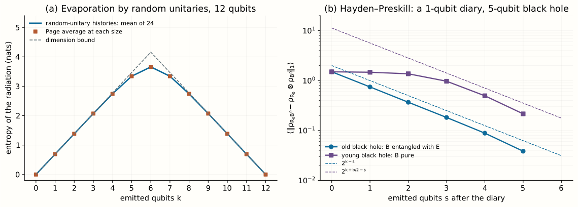
Model the black hole and its radiation by a random pure state of $K$ qubits, with $k$ of them in the radiation. By §5 the average entropy of the radiation is within half a nat of $\min (k,K-k)\log 2$ for all $k$: it rises with the number of emitted qubits until $k=K/2$ and then falls. This is the Page curve. The left panel of the figure in §7 compares it with the dimension bound for twelve qubits.

Page’s second paper asked when information appears in the radiation. The information in the radiation, in the sense of its deficit from maximal entropy, is

$$\mathcal{I}(R)=\log m-S(R)\simeq \frac{m}{2n},m\le n,$$

where $m=2^k$ is the dimension of the radiation and $n=2^{K-k}$ that of the black hole. It is exponentially small before the halfway point. After it the entropy follows the black hole, $S(R)\simeq \log n$, so $\mathcal{I}(R)\simeq \log (m/n)$ grows by two bits per emitted qubit, one because the radiation gains a qubit and one because its entropy decreases, until it reaches the full $K$ bits at the end. [Controlled perturbative.] That is, until the Page time the radiation is nearly maximally mixed, and any calculation perturbative in the inverse size of the black hole would find it exactly thermal, which was Page’s explanation of why the semiclassical calculation cannot see the information.

For a four-dimensional Schwarzschild black hole emitting photons and gravitons, Page later estimated that the maximum of the radiation entropy occurs after about $54$ per cent of the evaporation time, when the black hole has lost about $40$ per cent of its initial Bekenstein–Hawking entropy (Problem 11). [Stated only — refs: Page 2013.] The Page time is thus of the order of the evaporation time, and the black hole at that time is as semiclassical as it was at formation.

7. Black holes as mirrors

Hayden and Preskill asked how long a black hole keeps a secret. Alice throws a diary $A$ of $k$ qubits into a black hole $B$ of $b$ qubits; to track the information, the diary is maximally entangled with a reference $R_0$. Bob holds the earlier radiation $E$ and collects the next $s$ qubits of radiation, a system $Q$ of dimension $d_Q=2^s$. The black hole scrambles: its internal dynamics is modeled by a unitary $W$ on $AB$, drawn from the Haar measure, after which $AB$ splits into $Q$ and the remaining black hole $B^{\prime }$. Bob can recover the diary approximately, with an error controlled by the decoupling error, when $R_0$ is decoupled from $B^{\prime }$, that is, when ${\rho }_{R_0{B}^{\prime }}$ is close to ${\rho }_{R_0}\otimes {\rho }_{B^{\prime }}$. By Uhlmann’s theorem, the purification of ${\rho }_{R_0}\otimes {\rho }_{B^{\prime }}$ held by Bob can then be rotated into one that contains a copy of the maximal entanglement between $R_0$ and the diary. [Stated only — refs: Hayden–Preskill 2007; Hayden–Horodecki–Winter–Yard 2007.]

The decoupling can be computed with the Haar second moment. For any operator $Y$ on two copies of $AB$,

$${\mathbb{E}}_W[(W^{†}{)}^{\otimes 2}Y{W}^{\otimes 2}]={\mu }_{I}I+{\mu }_{F}F,$$

since the average commutes with all $W\otimes W$; the coefficients follow from the traces of $Y$ and $YF$. Take $Y=F_{B^{\prime }}\otimes I_{QQ}$, with $D=d_{B^{\prime }}{d}_Q$ the dimension of $AB$. Then $\mathrm{Tr}Y=d_{B^{\prime }}{d}_Q^2$ and $\mathrm{Tr}(YF)=d_{B^{\prime }}^2{d}_Q$, and

$${\mu }_I=\frac{d_{B^{\prime }}(d_Q^2-1)}{D^2-1},{\mu }_F=\frac{d_Q(d_{B^{\prime }}^2-1)}{D^2-1}.$$

The reference rides along, so the average purity of $R_0{B}^{\prime }$ is

$$\mathbb{E}\mathrm{Tr}{\rho }_{R_0{B}^{\prime }}^2={\mu }_I\mathrm{Tr}{\rho }_{R_0}^2+{\mu }_F\mathrm{Tr}{\rho }_{R_{0}AB}^2,$$

where the states on the right are those before the unitary. [Exact calculation, checked by sampling.] Since ${\rho }_{R_0}=I/d_{R_0}$ exactly, the squared Hilbert–Schmidt distance to the decoupled state is $\mathrm{Tr}{\rho }_{R_0{B}^{\prime }}^2-\mathrm{Tr}{\rho }_{B^{\prime }}^2/d_{R_0}$, whose average is ${\mu }_F(\mathrm{Tr}{\rho }_{R_{0}AB}^2-\mathrm{Tr}{\rho }_{AB}^2/d_{R_0})$. The trace norm on a space of dimension $d_{R_0}{d}_{B^{\prime }}$ obeys $\Vert X{\Vert }_1\le \sqrt{d_{R_0}{d}_{B^{\prime }}}\Vert X{\Vert }_2$, and with Jensen’s inequality

$$\mathbb{E}\Vert {\rho }_{R_0{B}^{\prime }}-{\rho }_{R_0}\otimes {\rho }_{B^{\prime }}{\Vert }_1\le \sqrt{d_{R_0}{d}_{B^{\prime }}{\mu }_F\left(\mathrm{Tr}{\rho }_{R_{0}AB}^2-\frac{\mathrm{Tr}{\rho }_{AB}^2}{d_{R_0}}\right)}.$$

[Proved.] Two cases give two answers.

The old black hole. After the Page time the black hole is maximally entangled with the early radiation $E$, so ${\rho }_B=I/d_B$, $\mathrm{Tr}{\rho }_{R_{0}AB}^2=1/d_B$ and $\mathrm{Tr}{\rho }_{AB}^2=1/D$. With $d_{R_0}=d_A=2^k$, $d_B=2^b$, $d_{B^{\prime }}=D/d_Q$ and ${\mu }_F\le 1/d_Q$, the bound becomes

$$\mathbb{E}\Vert {\rho }_{R_0{B}^{\prime }}-{\rho }_{R_0}\otimes {\rho }_{B^{\prime }}{\Vert }_1\le \frac{d_A}{d_Q}=2^{k-s}.$$

In fact a diary of $k$ qubits is returned once Bob has collected a few more than $k$ qubits, with an error that halves with each additional one, independently of the size of the black hole.

The young black hole. Before the Page time, take $B$ in a pure state. Then $\mathrm{Tr}{\rho }_{R_{0}AB}^2=1$, $\mathrm{Tr}{\rho }_{AB}^2=1/d_A$, and the bound becomes $2^{k+b/2-s}$: Bob must wait until more than half of the black hole has been emitted. [Exact calculation, from the bound.] The figure shows the average trace distance, sampled over Haar unitaries, for a one-qubit diary and a five-qubit black hole, together with the two bounds.

Checkpoint 2. In the old black hole, why does the early radiation $E$ make the return fast?

Answer. The black hole is maximally entangled with $E$, so Bob already holds a purification of most of its state. The unitary spreads the diary over all of $AB$, and a few emitted qubits, combined with $E$, suffice to purify the reference. Without $E$ the same information is spread over a system Bob does not hold, and he must collect more than half of it.

The model assumes that the black hole scrambles as fast as a Haar unitary. A real black hole scrambles in a time of order $\frac{\beta }{2\pi }\log S_{\mathrm{BH}}$, which Hayden and Preskill estimated and Sekino and Susskind argued is the shortest possible, so that black holes are the fastest scramblers in nature. [Stated only — refs: Hayden–Preskill 2007; Sekino–Susskind 2008.] Lecture 26 finds the same logarithm in the position of the quantum extremal surface.

8. Self-study: from ensembles to histories

The Page curve of §6 assigns an independent random state to each value of $k$. A family of ensembles is different from a history: the states at successive steps must be related by a common unitary process, with compatible records in the radiation. The left panel of the figure uses a dynamical model. At each step a random unitary acts on the qubits that remain in the black hole, and one of them is moved into the radiation. The unitary on the black hole does not change the entropy of the radiation, and the transfer changes it by at most $\log 2$. The mean over histories follows the Page average, and at twelve qubits individual histories stay close to it.

A realistic evaporation model adds constraints that change the curve. Energy conservation restricts the unitaries to energy shells and couples the rate of emission to the temperature; locality limits how fast the unitaries scramble; a black hole that starts in a mixed state, or entangled with a reference, has a different endpoint. Problem 13 builds one such model. The finite results used in the rest of the semester are the bound, the average near it, and the time at which information returns.

9. Self-study: why small corrections do not help

One might hope that small corrections to Hawking’s pair state, invisible in the semiclassical calculation, remove the conflict of §3. Mathur showed that corrections of small norm to each pair change the growth of the entanglement by a small amount per pair, so that the entropy of the radiation still grows: the Page curve requires order-one changes in the state of the late radiation, compared with the state of Hawking pairs. [Stated only — refs: Mathur 2009.] After the Page time a late outgoing quantum must be highly entangled with the early radiation, for the entropy to decrease, and also with its partner behind the horizon, for the horizon to be smooth. Strong subadditivity forbids both. Almheiri, Marolf, Polchinski and Sully concluded that one of the assumptions fails, possibly the smoothness of the horizon. [Stated only — refs: Almheiri–Marolf–Polchinski–Sully 2012.] Lectures 25–27 show how the gravitational entropy calculation evades the argument: after the Page time the partner belongs to the island, which is part of the entanglement wedge of the radiation, so the two entanglements are one.

10. What to take away

• Exact calculation: modes of positive frequency in the affine coordinate at the horizon pair each outgoing quantum with a partner inside, in a thermofield double at $\beta =2\pi /\kappa$; the outgoing quanta are thermal at $T_H=\kappa /2\pi$.
• Exact: in a unitary evaporation from a pure state, $S(R)\le S_{\mathrm{BH}}(t)$, and Hawking’s growing entropy violates this bound after the Page time, while the black hole is still large.
• Exact calculation: for a random pure state the average purity is $(m+n)/(mn+1)$, and the average entropy of two qubits is $\frac{1}{3}$.
• Controlled perturbative: at large $n$ the average entropy is $\log m-(m^2-1)/2mn$; Page’s exact formula is stated.
• Proved: in the Hayden–Preskill model the reference decouples from the remaining black hole within $2^{k-s}$ for an old black hole and $2^{k+b/2-s}$ for a young one.
• Stated only: a real black hole scrambles in a time of order $\frac{\beta }{2\pi }\log S_{\mathrm{BH}}$, and the Page time of a four-dimensional black hole is about $54$ per cent of its lifetime.

11. Looking ahead

Lecture 25 specifies a gravitational system in which the radiation entropy can be computed: Jackiw–Teitelboim gravity coupled to matter and to a flat bath that collects the radiation. Lecture 26 finds that the entropy of the baths contains a contribution from an island that contains the interior and reaches just outside the horizon, reproducing the bound $S(R)\le 2S_{\mathrm{BH}}$ of the two-sided black hole in equilibrium, and Lecture 27 derives the rule from replica geometries, whose two saddles are the gravitational counterparts of the two terms in the Haar purity of §5.

12. Problem set

Classroom core

1. The smaller subsystem. Explain why the bound of §4 involves $\min (m,n)$, and why it holds for mixed global states only in a weaker form.

2. A four-qubit protocol. Prepare two Bell pairs, emit one member of each, then both partners. Compute the sequence of entropies.

3. Trace the swaps. Derive $\mathbb{E}\mathrm{Tr}{\rho }_R^2=(m+n)/(mn+1)$ and identify the origin of each term.

4. The partner mode. Continue $(-\kappa U{)}^{i\omega /\kappa }$ from $U<0$ to $U>0$ through the lower half plane, and use the two annihilation conditions of §2 to show that $|0_U⟩$ has occupation $1/(e^{2\pi \omega /\kappa }-1)$ in the outgoing mode.

5. The first correction. Expand $S(I/m+\delta )$ to second order, derive $\mathbb{E}S=\log m-(m^2-1)/2mn+O(n^{-2})$, and compare with Page’s formula at $m=2$, $n=16$.

6. The Hayden–Preskill coefficients. Solve $\mathrm{Tr}({\mu }_{I}I+{\mu }_{F}F)=\mathrm{Tr}Y$ and $\mathrm{Tr}(({\mu }_{I}I+{\mu }_{F}F)F)=\mathrm{Tr}(YF)$ for $Y=F_{B^{\prime }}\otimes I_{QQ}$.

Self-study consolidation

7. Two qubits. With the density $3x^2$ for $x={\lambda }_1-{\lambda }_2$, verify the average purity $\frac{4}{5}$ and compute the average entropy $\frac{1}{3}$.

8. An invalid history. What is missing from a family of independent random states at each $k$, and what does the dynamical model of §8 add?

9. Page’s information. Show that $\mathcal{I}(R)=\log m-\mathbb{E}S(R)$ is below half a nat for $m\le n$ at large dimensions, and estimate how many qubits beyond the halfway point raise it to one bit.

10. The young black hole. Derive the bound $2^{k+b/2-s}$ from the general decoupling inequality with $B$ in a pure state.

11. The Page time in four dimensions. Assume that the radiation entropy grows at $1.4847$ times the rate at which the Bekenstein–Hawking entropy decreases, and that $M^3$ decreases linearly in time. Find the fraction of the initial entropy that remains at the Page time and the fraction of the lifetime that has elapsed.

12. Monogamy. For a qubit $b$ maximally entangled with a qubit $\tilde{b}$, show that $b$ is uncorrelated with any third system, and explain why this conflicts with a late Hawking quantum that is entangled both with its partner and with the early radiation.

Research extension

13. Energy-conserving evaporation. Build a random-unitary evaporation model with energy shells, a transfer rule tied to the temperature, and an initial mixed component. Known: the unrestricted Haar model gives the Page curve of §6; Page’s 2013 estimate uses a thermodynamic emission law. Completion: the entropy curve with its sampling uncertainty, compared with the unrestricted model after explaining the difference between the ensembles.

14. Scrambling by local circuits. Replace the Haar unitary of §7 by a brickwork circuit of two-qubit random gates on a line of $10$–$12$ qubits, and find the depth at which the decoupling bound of the old black hole is reached. Known: local circuits in one dimension scramble in a depth proportional to the number of qubits, and Sekino and Susskind argue that black holes scramble in a time logarithmic in their entropy. Completion: the decoupling distance as a function of depth, with the linear scaling identified.

15. The Petz decoder. Compute the Petz map of Lecture 20 for the channel from the reference-entangled diary to Bob’s systems $EQ$, with the maximally mixed reference state, and its recovery fidelity as a function of $s$. Known: decoupling implies the existence of a decoder by Uhlmann’s theorem, and Lecture 20 recalls the result of Barnum and Knill that the Petz map is nearly optimal. Completion: the fidelity for $k=1$, $b=3$, compared with the bound $1-2^{k-s}$.

13. Answer checkpoints

1. Both reduced states share the nonzero Schmidt spectrum, whose rank is at most the smaller dimension. For a mixed global state the Araki–Lieb inequality $|S(R)-S(B)|\le S(RB)$ replaces the equality, and $S(R)\le \min (\log m,\log n+S(RB))$.

2. $0,\log 2,2\log 2,\log 2,0$.

3. $\mathrm{Tr}{F}_R=m$ and $\mathrm{Tr}{I}_{B{B}^{\prime }}=n^2$ give $m{n}^2$; the swap term gives $\mathrm{Tr}(F_R^2)\mathrm{Tr}{F}_B=m^{2}n$. The first term contracts each copy with itself, the second exchanges the copies.

4. The continuation gives $e^{-\pi \omega /\kappa }(\kappa U{)}^{i\omega /\kappa }$. From $b|0⟩=e^{-\pi \omega /\kappa }{\tilde{b}}^{†}|0⟩$ and $\tilde{b}|0⟩=e^{-\pi \omega /\kappa }{b}^{†}|0⟩$, $⟨b^{†}b⟩=e^{-2\pi \omega /\kappa }⟨\tilde{b}{\tilde{b}}^{†}⟩=e^{-2\pi \omega /\kappa }(1+⟨b^{†}b⟩)$, using the symmetry of the state, and solving gives the Planck distribution.

5. $S=\log m-\frac{m}{2}\mathrm{Tr}{\delta }^2+O({\delta }^3)$ and $\mathbb{E}\mathrm{Tr}{\delta }^2=\frac{m^2-1}{m(mn+1)}$. At $m=2$, $n=16$ the correction gives $0.64627$, and Page’s formula ${\sum }_{17}^{32}\frac{1}{j}-\frac{1}{32}=0.64652$.

6. ${\mu }_I{D}^2+{\mu }_{F}D=d_{B^{\prime }}{d}_Q^2$ and ${\mu }_{I}D+{\mu }_F{D}^2=d_{B^{\prime }}^2{d}_Q$. Subtracting the first from $D$ times the second gives ${\mu }_F$, and then ${\mu }_I$.

7. $\mathbb{E}{x}^2=\frac{3}{5}$, so $\mathbb{E}\mathrm{Tr}{\rho }^2=\frac{4}{5}$. The integral ${\int }_0^{1}3x^{2}h(\frac{1+x}{2})dx$ equals $\frac{1}{3}$, which also equals $\frac{1}{3}+\frac{1}{4}-\frac{1}{4}$.

8. A common unitary process and compatible radiation records. In the dynamical model each state follows from the previous one by a unitary on the black hole and a transfer, so the entropies at successive steps differ by at most $\log 2$.

9. $\mathcal{I}\simeq m/2n\le \frac{1}{2}$ for $m\le n$. After the halfway point $S(R)\simeq \log n$ and $\mathcal{I}\simeq \log (m/n)=(2k-K)\log 2$, so one bit is exceeded at the first emission after the halfway point.

10. $\mathrm{Tr}{\rho }_{R_{0}AB}^2=1$ and $\mathrm{Tr}{\rho }_{AB}^2=1/d_A$ give ${\mu }_F(1-1/d_A^2)\le 1/d_Q$, and $\sqrt{d_A{d}_{B^{\prime }}/d_Q}=d_A\sqrt{d_B}/d_Q=2^{k+b/2-s}$.

11. $S_{\mathrm{rad}}=1.4847(S_0-S_{\mathrm{BH}})$ equals $S_{\mathrm{BH}}$ when $S_{\mathrm{BH}}/S_0=1.4847/2.4847=0.5975$. With $S\propto M^2$ and $M^3\propto t_{\mathrm{evap}}-t$, the elapsed fraction is $1-0.5975^{3/2}=0.538$.

12. The reduced state of $b\tilde{b}$ is pure, so the state of $b\tilde{b}$ and any third system is a product. A late quantum after the Page time must purify part of the early radiation and must also be purified by its partner, and strong subadditivity forbids both.

Wiki connections. Page curve