Lecture 32 — The full chain from information to geometry

The course followed one question through thirty-one lectures: what can an observer who has access to part of a system know and recover, and when does the answer take the form of a geometry? We began with algebras of observables in finite systems, where every statement is a theorem, passed to the continuum, where algebras change type and modular flows become geometric, and only then met the holographic dictionary, black holes and the algebras of large-$N$ theories. This lecture retraces the chain in six links, each with an exact statement and the assumption that the next link adds. It compares three entropy formulas that look alike, the code formula with a central term, the Ryu–Takayanagi formula for an interval and the generalized entropy of an island, and finds that their status differs at every step. It follows one algebraic cancellation through a finite code and through the relative-entropy identity of holography, and one modular clock from an entangled pair to the emergent time of Lecture 31. It ends with the audit of an overstated conclusion, with projects that can be completed, and with the questions that remain open where the course stops.

How to use this lecture

Classroom core, one meeting of three hours. The history (§1, 10 minutes), the chain in six links (§2, 35 minutes), and three entropy formulas (§3, 25 minutes) come before a 10-minute break. After it come one cancellation with two uses (§4, 20 minutes), one clock and two clocks (§5, 20 minutes), and the audit of a conclusion (§6, 20 minutes), with 40 minutes for Checkpoints 1 and 2 and Problems 4–6; Problems 1–3 complete the core assignment. These allocations are proposals and have not been tested in class. The lecture works best as a workshop in which students reconstruct the arguments from their notes, which they may consult throughout.

Self-study. Final projects with their deliverables (§7), questions at the boundary of the course (§8), and Problems 7–12, including the three algebras of a boundary theory, the origin of the factor $2\pi$ and the comparison of Rehren’s map with reconstruction.

Research extension. Three of the projects of §7, as Problems 13–15.

Prerequisites. The whole course, and in particular Lecture 3 for the modular operator of an entangled pair, Lecture 4 for codes with sectors, Lecture 10 for the Bisognano–Wichmann theorem, Lecture 16 for the entropy of an interval, Lecture 21 for the relative-entropy identity, Lectures 25 and 26 for the island, and Lectures 28–31 for the algebras of the last block.

What this lecture establishes. It proves nothing new. It collects the results of Lectures 1–31 with the status that each lecture assigned them, recomputes the modular composition for the two orientations of Lectures 30 and 31, and sets the three entropy formulas side by side with the assumptions that each requires.

0. Reading

Primary.

• D. Harlow, TASI Lectures on the Emergence of the Bulk in AdS/CFT (2018).
• A. Almheiri, T. Hartman, J. Maldacena, E. Shaghoulian, A. Tajdini, The entropy of Hawking radiation (2020).
• H. Liu, Lectures on entanglement, von Neumann algebras, and emergence of spacetime (2025).

Secondary.

• E. Witten, Notes on Some Entanglement Properties of Quantum Field Theory (2018).
• A. Almheiri, X. Dong, D. Harlow, Bulk Locality and Quantum Error Correction in AdS/CFT (2014).
• M. Rangamani, T. Takayanagi, Holographic Entanglement Entropy (2016).

Optional research reading.

• J. Sorce, Notes on the type classification of von Neumann algebras (2023).
• D. Harlow, Jerusalem Lectures on Black Holes and Quantum Information (2014).
• X. Dong, D. Harlow, A. C. Wall, Reconstruction of Bulk Operators within the Entanglement Wedge in Gauge-Gravity Duality (2016).
• J. Cotler, P. Hayden, G. Penington, G. Salton, B. Swingle, M. Walter, Entanglement Wedge Reconstruction via Universal Recovery Channels (2017).

1. What did the course connect?

The ideas of the course arrived in an order different from the one we followed. Bekenstein’s entropy of 1972 and Hawking’s radiation of 1974 posed the problem; Maldacena’s conjecture of 1997 and the dictionary of Gubser, Klebanov, Polyakov and Witten in 1998 gave a framework in which it could be asked precisely. Rehren’s algebraic holography of 1999 showed that part of the correspondence follows from symmetry and causality alone. Ryu and Takayanagi related entropy to area in 2006, and Van Raamsdonk argued in 2010 that entanglement builds connectivity. In the years that followed the program acquired its quantum-information form. Lashkari, McDermott and Van Raamsdonk derived the linearized Einstein equations from the entanglement first law, and Faulkner, Guica, Hartman, Myers and Van Raamsdonk extended the derivation to every dimension, in 2013–14; Almheiri, Dong and Harlow found the error-correcting codes in 2014, and Jafferis, Lewkowycz, Maldacena and Suh the relative-entropy identity in 2015. In 2019 the quantum extremal surfaces of Penington and of Almheiri, Engelhardt, Marolf and Maxfield, the island rule of Almheiri, Mahajan, Maldacena and Zhao, and the replica wormholes that justify them produced the Page curve from a gravitational calculation. Since 2021 the algebras themselves have become the object: the emergent type III${}_1$ algebras and times of Leutheusser and Liu, the crossed products of Witten, and the algebras of observers of Chandrasekaran, Longo, Penington and Witten.

We took the algebraic structures first, in finite systems where every statement can be proved, then the continuum, where the structures change character, then the dictionary, and only at the end the gravitational applications. The order was chosen so that each holographic statement would arrive with a finite or continuum counterpart already understood, and so that the student could see where a theorem ends and a proposal begins.

2. The chain in six links

The figure shows the six blocks of the course and the assumption that each arrow adds. We take them in turn, with one exact statement from each and its status as the lecture assigned it.

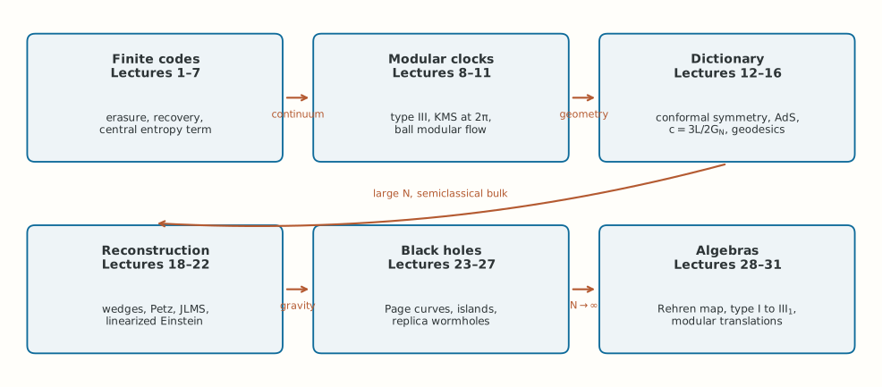
Finite codes, Lectures 1–7. A logical qutrit encoded in three qutrits can be recovered from any two shares and from no single one (Lecture 2), and in a code with sectors and fixed auxiliary states the entropy of a region is

$$S({\rho }_A)=S_{\mathcal{M}}(\rho )+⟨\mathcal{L}{⟩}_{\rho },S_{\mathcal{M}}(\rho )=H(p)+\sum _{\alpha }{p}_{\alpha }S({\rho }_{\alpha }),\mathcal{L}=\underset{\alpha }{⨁}S({\chi }_{\alpha })I_{\alpha },$$

with $\mathcal{L}$ central in the reconstructed algebra $\mathcal{M}$ (Lectures 4 and 21). [Proved.] The modular operator of an entangled pair is $\Delta ={\rho }_A\otimes {\rho }_B^{-1}$ (Lecture 3). The arrow to the next block adds the continuum: infinitely many degrees of freedom, for which the algebras of regions need not be of type I.

Modular clocks, Lectures 8–11. The entropy of an interval of a lattice field diverges as the spacing goes to zero, while the mutual information of separated intervals converges (Lecture 8, numerical in a defined model). The local algebras of a quantum field theory are of type III${}_1$ under nuclearity and scaling hypotheses (Lecture 9, hypothesis-explicit), and the modular flow of a Rindler wedge in the vacuum is the boost at rapidity $2\pi s$ (Lecture 10, stated), with the Unruh temperature $a/2\pi$ as an exact consequence. The modular flow of a ball in a conformal field theory is the conformal image of the boost (Lecture 11, exact calculation of the map, stated for the flow), and the first law $\delta S=\delta ⟨K⟩$ is the stationarity of relative entropy (Lecture 11, proved). The arrow adds geometry: conformal symmetry, whose group is the isometry group of AdS.

The dictionary, Lectures 12–16. The conformal algebra is the isometry algebra of AdS${}_{d+1}$ (Lectures 12–13, exact). Normalized single-trace operators of a large-$N$ theory have connected $n$-point functions of order $N^{2-n}$ and become generalized free fields (Lecture 14, exact calculation in the Gaussian model). The scalar two-point function follows from the regularity of a bulk solution and a counterterm (Lecture 15, exact calculation within the dictionary of Gubser, Klebanov, Polyakov and Witten, which is stated). The entropy of an interval, $\frac{c}{3}\log (\ell /ϵ)$, equals the length of a geodesic divided by $4G_3$ with $c=3L/2G_3$ (Lecture 16: both sides exact, their identification the Ryu–Takayanagi prescription, stated). The arrow adds large $N$ and a semiclassical bulk: a code subspace on which bulk fields are free to leading order.

Reconstruction, Lectures 18–22. A free field in AdS${}_2$ is a smeared boundary operator (Lecture 18, exact calculation), and the center of global AdS${}_3$ has representatives on every pair of three arcs that agree on a code subspace (Lecture 18, formal analogy, exact in the three-qutrit code). Entanglement wedges contain causal wedges (Lecture 19, sketched under the null energy condition) and change discontinuously, as in the two-interval transition at $b/\ell =\sqrt{2}-1$ (Lecture 19, exact at leading order). Petz’s theorem turns preserved relative entropy into a decoder (Lecture 20, model proof). A formula with a central area operator implies the equality of boundary and bulk relative entropies (Lecture 21, proved in codes, sketched in holography). The first law for all intervals implies the linearized Hamiltonian constraint for static perturbations of AdS${}_3$ (Lecture 22, proved under analyticity), and with all Lorentz frames the linearized Einstein equations (stated). The arrow adds gravity: dynamical geometry, horizons and black holes.

Black holes, Lectures 23–27. The modular operator of the thermofield double is $e^{-\beta (H_R-H_L)}$, and its flow is the boost of the Kruskal plane (Lecture 23, exact). The Hawking–Page transition and Cardy’s formula follow from Euclidean actions (Lecture 23, exact calculation). The average entropy of a subsystem of a random pure state follows the Page curve (Lecture 24, exact for the purity, controlled at large dimension for the entropy). The JT model with a bath has an exact Hartle–Hawking state, and the generalized entropy of an island is an explicit function whose extremum gives the late-time entropy $2S_{\mathrm{BH}}+\frac{c}{3}(b+\log 2)$ (Lectures 25–26, exact for the functional, controlled at large ${\phi }_r/c$). The island rule itself is stated, and its replica derivation is sketched under explicit hypotheses (Lecture 27). The arrow adds the limit $N\to \infty$, in which the algebras of the boundary change type.

Algebras, Lectures 28–31. On a fixed AdS, wedges correspond to boundary diamonds, and any net transfers with its modular structure (Lecture 28, proved in AdS${}_3$); a Haag-dual, strongly additive boundary net with factor diamond algebras leaves nothing at the center of three arcs (Lecture 28, proved). In thermal AdS the large-$N$ algebra is of type I, and in the black-hole phase decaying correlators exclude a type I factor (Lecture 29, proved), with type III${}_1$ stated. Nested algebras with a half-sided modular inclusion generate a translation with positive generator (Lecture 30, Borchers sketched, Wiesbrock stated), and in the JT model this translation carries boundary operators across the future horizon (Lecture 31, exact).

3. Three entropy formulas

Three formulas of the course look alike. Each is an entropy written as the sum of a term that plays the role of an area and a term that counts quantum entropy, and each was derived with different means. Set them side by side:

$$\begin{array}{rlrl}& \text{a code with sectors (Lectures 4, 21):}& & S({\rho }_A)=⟨\mathcal{L}{⟩}_{\rho }+S_{\mathcal{M}}(\rho ),\\ & {\text{an interval in AdS}}_3\text{ (Lecture 16):}& & S_A=\frac{\mathrm{Length}({\gamma }_A)}{4G_3}=\frac{c}{3}\log \frac{\ell }{ϵ},\\ & \text{an island in JT (Lectures 25, 26):}& & S_{\mathrm{gen}}(a)=S_0+\frac{{\phi }_r}{a}+\frac{c}{6}\log \frac{(a+b{)}^2}{aϵ}.\end{array}$$

In the code, the area term $⟨\mathcal{L}{⟩}_{\rho }$ is the entropy of the auxiliary states that the encoding attaches to each sector. It is central by construction, and the formula is a theorem about tensor products and direct sums, valid for every state of the code. In the interval, both sides are exact calculations, the entropy of a two-dimensional conformal field theory from twist operators and the length of a geodesic of AdS${}_3$, and their equality with $c=3L/2G_3$ is a test of the Ryu–Takayanagi prescription; the bulk entropy term is absent at this order. In the island, the area term $S_0+{\phi }_r/a$ is the dilaton at the endpoint, the matter term is the entropy of the matter on the union of the island and the radiation in the state of the model, and the formula is exact as a function of $a$. Its extremum is the entropy of the radiation only by the island rule, a prescription whose derivation from replica wormholes assumes a dominant replica-symmetric saddle and its continuation in $n$.

The resemblance is therefore real and instructive, and the statuses differ at each step. The code formula needs no extremization, because the code fixes the region; the interval formula extremizes a classical length; the island formula extremizes a generalized entropy, and then compares saddles. In the code the area term is an operator; in holography it becomes an operator only at the order at which the area fluctuates, which is how Lecture 21 connected the two.

Checkpoint 1. Which of the three formulas is a theorem about a quantum system, which is a test of a prescription, and which needs a rule to become an entropy?

Answer. The code formula is a theorem about the code. The interval formula equates two exact calculations, and the equality tests the Ryu–Takayanagi prescription. The island formula is an exact function whose extremum becomes the entropy of the radiation through the island rule, which is stated, with a derivation sketched under explicit hypotheses.

4. One cancellation, two uses

The same cancellation appears twice. In a code with sectors, relative entropy is the difference of modular energy and entropy, and the central term cancels between them:

$$D({\rho }_A\Vert {\sigma }_A)=\Delta ⟨\mathcal{L}+K_{\mathcal{M}}^{\sigma }⟩-\Delta ⟨\mathcal{L}⟩-\Delta S_{\mathcal{M}}=D_{\mathcal{M}}(\rho \Vert \sigma ).$$

[Proved (Lecture 21).] By Petz’s theorem of Lecture 20, preserved relative entropy is equivalent to the existence of a decoder, so the algebra $\mathcal{M}$ is recoverable from $A$. In holography, the formula of Faulkner, Lewkowycz and Maldacena gives a modular Hamiltonian of the form $\widehat{\mathrm{Area}}/4G_N+K_{\mathrm{bulk}}$ at leading order, and the same cancellation gives the relative-entropy identity of Jafferis, Lewkowycz, Maldacena and Suh. [Sketched (Lecture 21).] Combined with the approximate recovery theorems, it gives the reconstruction of the entanglement wedge. [Stated only — refs: Dong–Harlow–Wall 2016; Cotler et al. 2017.]

The algebra is the same in both uses, and the status is not. In the code the cancellation is exact for every state. In holography it holds at leading order in $G_N$, for states in a code subspace whose size must be controlled, and the decoder is approximate. The finite model shows what the identity means, and whether holography has it is a separate question, answered at leading order.

5. One clock, two clocks

A single modular operator gives a clock, and the course met it in four settings. For an entangled pair, $\Delta ={\rho }_A\otimes {\rho }_B^{-1}$ (Lecture 3). For a Rindler wedge in the vacuum, $\Delta =e^{-2\pi K}$ with $K$ the boost (Lecture 10). For a ball in a conformal field theory, the flow is the conformal Killing flow $\zeta$ (Lecture 11), and in the bulk it is the AdS–Rindler boost of Lecture 22, exactly so on a fixed AdS by Lecture 28. For the thermofield double, $\Delta =e^{-\beta (H_R-H_L)}$, the Killing flow of the black hole (Lecture 23). In each geometric case the flow is a boost, which fixes the edge of its region, and its orbits approach the horizon without crossing it.

Two modular operators can do what one cannot. For nested half-lines with a common vacuum, Lectures 30 and 31 found

$${\Delta }_{\mathcal{A}(0,\infty )}^{-is}{\Delta }_{\mathcal{A}(b,\infty )}^{is}=U(b(e^{2\pi s}-1)),{\Delta }_{\mathcal{A}(-\infty ,0)}^{-is}{\Delta }_{\mathcal{A}(-\infty ,-b)}^{is}=U(b(1-e^{-2\pi s})),$$

which are the same formula with $b\to -b$ and $s\to -s$, since the second configuration is the reflection of the first. [Exact (Problem 5).] The composition of two boosts about different points is a translation, which has no fixed point at the edge and moves operators across it. In the JT model of Lecture 31 the second formula is a Kruskal translation, built from two boundary modular operators, which carries outgoing operators of the right boundary into the black-hole interior.

The factor $2\pi$ runs through the whole chain. It is the KMS period of the boost in Lecture 10, the Hawking temperature $1/2\pi$ in the units of Lecture 25, and the factor in $e^{2\pi s}$ that maps the modular strip of width $\frac{1}{2}$ onto the upper half-plane of positive energy in Borchers’ theorem (Lecture 30). These are one fact seen three times: the modular flow of a wedge is a boost, and the boost of a horizon is thermal at $\beta =2\pi$ in the units of its surface gravity.

Checkpoint 2. Why can a single modular flow never move an operator across the edge of its region, while two can?

Answer. A modular flow maps the algebra to itself, and in the geometric cases it acts as a boost or dilation that fixes the edge, so orbits approach it and never cross. Two flows with different fixed points compose into a translation, which moves the edge itself.

6. Audit a conclusion

Consider the statement:

“The Page curve, the type III${}_1$ algebras and the reconstruction maps together prove that spacetime is a quantum error-correcting code.”

Each component has a precise status. Unitarity forces the entropy of radiation emitted from a pure state to obey $S(R)\le S_{\mathrm{BH}}(t)$ and to return to zero (Lecture 24, exact); the Page curve is the typical behavior, with an exact average purity and an average entropy controlled at large dimension (Lecture 24). Its gravitational derivation uses the island rule, stated, and replica wormholes, sketched under hypotheses (Lectures 26–27). Type III${}_1$ algebras are a property of continuum quantum field theory at every $N$, under the hypotheses of Lecture 9; the large-$N$ algebra of the black-hole phase is provably not of type I, and its type III${}_1$ is stated (Lecture 29). Reconstruction maps are theorems in codes (Lectures 2, 20, 21), exact calculations for free fields on fixed AdS (Lecture 18), and leading-order statements in holography (Lecture 21). And “spacetime is a code” is a formal analogy, exact in finite models and valid in holography on a code subspace, to the order at which the bulk effective theory holds (Lecture 18).

A conclusion with the same content and the right status reads as follows. In holographic theories at large $N$, semiclassical bulk observables behave as encoded information on a code subspace, relative entropy controls their recovery, and modular structure organizes geometric flows, including flows that cross horizons; finite codes and continuum models show which parts of this can be proved, and where the proof stops. The revised statement is narrower, and it can be tested.

7. Self-study: final projects

Each project ends in a calculation that someone else can check, a script or a derivation, and a paragraph on what would limit or falsify its interpretation. A literature summary without a calculation does not complete a project.

A. An imperfect code. Use the deformed encoding of Lecture 7. Compare the explicit decoder, the Petz decoder of Lecture 20 and the universal recovery bound, as functions of the deformation. Deliver the encoding, one analytic derivation, tests with a reference system, and the region of exact recovery.

B. A regulated field. Use the oscillator chain of Lecture 8. Study the mutual information of separated intervals while varying the spacing, the mass and the size of the box independently. Deliver the covariance construction, the evidence of convergence, and an explanation of why the calculation does not classify the continuum algebra.

C. A complete scalar dictionary. Extend Lecture 15 to an integer value of $\nu$, where logarithms and a scheme-dependent contact term appear, or to a massive vector. Deliver the radial solution, the boundary expansion, the counterterms, the response and the separated-point correlator, with the normalization fixed throughout.

D. Competing entropy surfaces. Extend the two-interval transition of Lecture 19 or the island of Lecture 26 to a case not treated there, such as the island at finite temperature with an asymmetric pair of baths. Deliver both candidate entropies, the extremality conditions in every varied coordinate, and an estimate of the regime of validity.

E. Modular translations. Use the chiral current of Lecture 30. Compute the modular group of an interval as a one-particle operator, verify that the three modular generators of a standard inclusion close into the Lie algebra of $PSL(2,\mathbb{R})$, and quantify the failure of the relation $i[K,P]=2\pi P$ under truncation.

F. The type of a large-$N$ algebra. Use the spectral densities of Lecture 29. Construct a finite model whose level density approaches the BTZ density, and measure the time at which its correlator departs from the infinite-$N$ decay, as a function of the number of levels.

8. Self-study: questions at the boundary of the course

Several questions are open where the course stops, and the course supplies the language in which to pose them. How large can a code subspace become before a single recovery map fails, and what replaces it beyond that size? How should the gravitational dressing of operators, and the central elements it produces, be organized beyond leading order in $G_N$, where Lecture 31 found that the half-sided inclusions of type III${}_1$ cannot survive unchanged? Which limiting algebras retain enough of the microscopic theory to describe times of the order of $e^S$, where the decay of Lecture 29 must stop? How does a quantum extremal surface translate into an efficient decoding procedure? And when do modular relations determine more than the causal structure of Lecture 31: a conformal factor, a proper time, a metric?

These are research questions, and the distinction between what was proved and what was proposed is what makes them precise.

9. What to take away

• Proved, in finite codes: a code with sectors has $S({\rho }_A)=S_{\mathcal{M}}(\rho )+⟨\mathcal{L}{⟩}_{\rho }$ with $\mathcal{L}$ central, and the relative entropies of $A$ and of $\mathcal{M}$ are equal; Petz’s theorem turns the equality into a decoder.
• Stated, with exact consequences: the vacuum modular flow of a wedge is a boost with KMS period $2\pi$ in rapidity, and that of a ball is its conformal image; the Unruh temperature and the modular vector of the ball are exact calculations.
• Exact, within prescriptions: the interval entropy matches a geodesic length, and the island functional has an explicit extremum; the Ryu–Takayanagi prescription and the island rule are stated, and the replica derivations are sketched under hypotheses.
• Proved, in the last block: the region map of AdS${}_3$ and the transfer of nets through it (the correspondence in general dimension is stated), the triviality of the three-arc intersection for Haag-dual, strongly additive nets with factor diamond algebras, the exclusion of a type I factor by decaying correlators, and the absence of half-sided inclusions in finite dimensions; the Kruskal translation of Lecture 31 is exact.
• Method: a holographic statement is as strong as its weakest link, and every link of the chain has a label that says how strong it is.

10. Looking ahead

The course ends here, and three continuations are natural. The AQFT course develops the algebraic tools, from Tomita–Takesaki theory to crossed products, in the generality that this course used in examples. The open questions of §8 are active research. And the first-semester synthesis, Lecture 17, can now be reread with the second semester in view: the recoverable observable of its title has become, by Lecture 31, an algebra whose modular structure produces a direction of time.

11. Problem set

Classroom core

1. One proof. Reproduce the proof that a formula $S({\rho }_A)=S_{\mathcal{M}}(\rho )+⟨{\mathcal{L}}_A{⟩}_{\rho }$ with ${\mathcal{L}}_A$ central implies $D({\rho }_A\Vert {\sigma }_A)=D_{\mathcal{M}}(\rho \Vert \sigma )$ (Lecture 21).

2. One calculation. Compute $d_0(s)\circ d_b(-s)$ for dilations of the line about $0$ and $b$, with the sign convention of the course, and state which modular operators implement it.

3. The status of the island. Is the formula $a_{\ast }=\frac{1}{2}(b+k+\sqrt{b^2+6bk+k^2})$ of Lecture 26 exact? State precisely of what it is the exact extremum and what further rule makes it an entropy.

4. Three area terms. For each formula of §3, identify the term that plays the role of an area, its origin, and whether it is an operator.

5. Two orientations. Compute the two products of modular unitaries of §5 by following the localization of an operator, and show that they are related by $b\to -b$, $s\to -s$.

6. Audit. Rewrite the statement “Lecture 31 shows that the boundary Hamiltonian evolves operators into the black-hole interior” so that it is correct, and attach a status label to each part.

Self-study consolidation

7. Finite $N$ and finitely many degrees of freedom. Is a conformal field theory at finite $N$ a system with finitely many degrees of freedom? Answer with the three algebras of Lecture 29, §7.

8. An incomplete decoder test. A proposed decoder reproduces all logical populations in a basis. What is still untested, and what test is sufficient?

9. A small correction near a crossing. Use the shift $\delta (b/\ell )\simeq 3\delta S_{\mathrm{bulk}}/(2\sqrt{2}c)$ of Lecture 19 to explain why a correction of order one can change which entanglement wedge applies.

10. The factor $2\pi$. Trace the factor $2\pi$ through the KMS period of Lecture 10, the Hawking temperature of Lecture 25 and the dilation $e^{2\pi s}$ of Lecture 30, and explain why they are the same fact.

11. Which algebra is of type III${}_1$? Classify the type of the full algebra of a boundary theory on a sphere at finite $N$, the algebra of a boundary diamond, and the large-$N$ single-trace algebra below and above the Hawking–Page temperature, with the status of each claim.

12. Rehren and reconstruction. What does Rehren’s correspondence of Lecture 28 give that entanglement-wedge reconstruction does not, and what does reconstruction give that Rehren’s correspondence does not?

Research extension

13. Project D. Known: the zero-temperature island of Lecture 26 and the late-time island of the two-sided equilibrium. Completion: the island at finite temperature with two baths at different distances $b_L\ne b_R$, its extremality conditions, the Page time, and an estimate of the regime of validity.

14. Project E. Known: Wiesbrock’s theorem relates a standard half-sided modular inclusion to a Möbius-covariant net. Completion: the modular generator of $\mathcal{A}((0,1))$ for the chiral current as an explicit one-particle operator, and a symbolic check that it closes with the dilations about $0$ and $1$ into $\mathfrak{sl}(2,\mathbb{R})$.

15. Project F. Known: the BTZ spectral density of Lecture 29 and the late-time plateau of Lecture 23. Completion: a finite model with $N$ levels whose density approaches the BTZ density, the time at which its correlator departs from the infinite-$N$ decay, and the scaling of that time with $N$.

12. Answer checkpoints

1. Differentiating the formula at $\sigma$ along traceless $\delta \rho$ gives $V^{†}{K}_A^{\sigma }V={\mathcal{L}}_A+K_{\mathcal{M}}^{\sigma }$ on the code, the constant fixed at $\rho =\sigma$. Then $D=\Delta ⟨K⟩-\Delta S$ for both $A$ and $\mathcal{M}$, and $\Delta ⟨{\mathcal{L}}_A⟩$ cancels.

2. $d_0(s)\circ d_b(-s)(u)=u+b(e^{2\pi s}-1)$. With $\mathcal{M}=\mathcal{A}((0,\infty ))$ and $\mathcal{N}=\mathcal{A}((b,\infty ))$ in the vacuum, it is implemented by ${\Delta }_{\mathcal{M}}^{-is}{\Delta }_{\mathcal{N}}^{is}$.

3. It is the exact extremum of the generalized-entropy functional of Lecture 25 at zero temperature, a semiclassical expression. It becomes the entropy of the radiation through the island rule, which is stated, after comparison with the no-island saddle.

4. Code: $⟨\mathcal{L}⟩$, the entropy of the auxiliary states, a central operator. Interval: the geodesic length over $4G_3$, a classical quantity at this order. Island: $S_0+{\phi }_r/a$, the dilaton at the endpoint, which becomes an operator only when the dilaton is quantized.

5. For $(0,\infty )\supset (b,\infty )$, $w\mapsto b+e^{-2\pi s}(w-b)\mapsto w+b(e^{2\pi s}-1)$. For $(-\infty ,0)\supset (-\infty ,-b)$, $w\mapsto -b+e^{2\pi s}(w+b)\mapsto w+b(1-e^{-2\pi s})$. Replacing $b\to -b$ and $s\to -s$ in the first gives $-b(e^{-2\pi s}-1)=b(1-e^{-2\pi s})$.

6. “In the JT model with a bath, at $G_N\to 0$ and in the Hartle–Hawking state, the modular operators of two algebras of boundary operators, all times and times before $t_0$, generate a Kruskal translation that moves outgoing boundary operators across the future horizon (exact). The boundary Hamiltonian generates the boost and does not (exact). The large-$N$ version is the proposal of Leutheusser and Liu (stated).”

7. No. The full algebra at finite $N$ is of type I with a discrete spectrum, but the theory has infinitely many modes, and the algebra of a diamond is of type III${}_1$ at every $N$ under the hypotheses of Lecture 9; only the large-$N$ single-trace algebra changes type with the limit.

8. Coherences between logical basis states and entanglement with a reference. A sufficient test is the action on a spanning set of matrix units, or the recovery of a maximally entangled state with a reference.

9. Near the crossing the two candidate entropies differ by an amount of order $c\delta (b/\ell )$, which is comparable to an order-one bulk entropy when $\delta (b/\ell )\sim 1/c$. A small correction then decides which surface has the smaller entropy.

10. The vacuum modular flow of a wedge is the boost at rapidity $2\pi s$, so a uniformly accelerated observer sees KMS period $2\pi /a$; a horizon with surface gravity $\kappa$ has temperature $\kappa /2\pi$; and Borchers’ theorem needs $e^{2\pi s}$ because the modular strip of width $\frac{1}{2}$ maps onto the upper half-plane under $a=e^{2\pi z}$. All three express that modular flow of a wedge is a boost with period $2\pi$ in imaginary rapidity.

11. Full algebra at finite $N$: type I (proved for a discrete spectrum with trace-class $e^{-\beta H}$). Diamond: type III${}_1$ (hypothesis-explicit). Large-$N$ algebra below the transition: type I (proved, Lecture 29). Above: a factor not of type I (proved), type III${}_1$ (stated).

12. Rehren’s map is exact, needs no large $N$ or code subspace, and carries the full modular structure, but it lives on a fixed geometry and its compact-region algebras may be trivial. Reconstruction applies to entanglement wedges that depend on the state and reaches deep regions, but holds at leading order on a code subspace.

Wiki connections. Ryu–Takayanagi formula · Page curve · type III₁ von Neumann algebras · crossed product