Mini-Lecture IV.6: White’s Bridge and the Contact Term

We study a normalized approximate identity and a test-function limit. The worked calculation and its limitations are the classroom target; the longer source reconstruction supports independent study.

How to use this lecture

Prerequisites: IV.5; the distribution bridge. Review the relevant prerequisite bridge before starting.

• Classroom core, 90 minutes: question and prerequisites (10); a normalized approximate identity and a test-function limit (25); worked calculation or laboratory (30); problems 1–2 (20); written exit check (5).
• Self-study, approximately 2–3 hours: reconstruct the algebra in the main text, work through the laboratory, then solve problems 1–3 before reading the answer checkpoints. The estimate is provisional.
• Research extension: problem 4 states the source-dependent task and what counts as completion. Its open claims are not assumed in the classroom assessment.

The classroom result is the explicitly calculated model or conditional derivation below. Retained sections marked Source reconstruction explain the IAS argument and identify provenance; that label does not certify the argument. The claim map records the research limits. The literal extended-surface identity fails the circle check in III.5; geometric QCD conclusions depending on it remain conditional.

Reading

• Primary: IAS lectures, pages 106-108. Consult the page images when an equation is clipped or extraction is ambiguous.
• Gentler route: the prerequisite bridges, followed by this lecture’s worked calculation.
• Optional research: the bibliography and version map identifies the primary papers for this module and their role.

Source Pages

Primary source: IASQCDLectures.pdf, pages 106-108.

The question

Large mass suppresses long paths. Under what conditions does the surviving contribution become a four-dimensional delta function with the coefficient required by the loop equation? Localization, normalization, and identification with the actual determinant are three separate checks.

What the bridge argument supplies

The source uses a narrow bridge between two spanning pieces to compare a connected fermion path touching the boundary twice with the contact splitting term. A geodesic obeys ${\ell }_{\mathrm{geo}}(x,y)\ge |x-y|$. Hence a weight bounded by $e^{-2m{\ell }_{\mathrm{geo}}}$ is also bounded by $e^{-2m|x-y|}$. This shows suppression away from the diagonal.

It does not determine the prefactor, the power of $m$, the ambient measure, or the exact radial kernel. Nor does weak convergence of bridged surfaces by itself imply pointwise alignment of tangent tensors. Those are additional ingredients in a derivation of the contact term.

Exact normalization in four dimensions

Test the kernel printed in the source:

$$q_m(x)=4m^4{e}^{-2m|x|}.$$

The unit three-sphere has area $2{\pi }^2$, so

$${\int }_{{\mathbb{R}}^4}{q}_m(x)d^{4}x=8{\pi }^2{m}^4{\int }_0^{\infty }{r}^3{e}^{-2mr}dr=8{\pi }^2{m}^4\frac{3!}{(2m{)}^4}=3{\pi }^2.$$

With ordinary Lebesgue measure it approaches $3{\pi }^2{\delta }^{(4)}$, not a unit delta. A unit approximate identity is

$$k_m(x)=\frac{4m^4}{3{\pi }^2}{e}^{-2m|x|}.$$

If the source intends a differently normalized integration measure, that convention and its effect on the coupling must be stated explicitly.

Proving the distributional limit

Let $\phi$ be a smooth compactly supported test function. Substitute $y=mx$:

$$\int k_m(x)\phi (x)d^{4}x=\frac{4}{3{\pi }^2}\int e^{-2|y|}\phi (y/m)d^{4}y.$$

The integrable majorant is a constant times $e^{-2|y|}$, so dominated convergence gives $\phi (0)$ as $m\to \infty$. This is the precise statement $k_m\to {\delta }^{(4)}$. A pointwise limit away from zero would be insufficient, since it cannot distinguish a unit delta from any multiple of one.

The first odd moments vanish by symmetry. The radial second moment is

$$\int |x{|}^2{k}_m(x)d^{4}x=\frac{5}{m^2},\int x_{\mu }{x}_{\nu }{k}_m(x)d^{4}x=\frac{5}{4m^2}{\delta }_{\mu \nu }.$$

Taylor expansion of a test function therefore yields

$$\int k_m\phi =\phi (0)+\frac{5}{8m^2}\Delta \phi (0)+O(m^{-4})$$

when sufficiently many bounded derivatives are available. For $\phi =e^{-a|x{|}^2}$ the leading correction is $-5a/m^2$, since $\Delta \phi (0)=-8a$. This gives a quantitative convergence check.

Tensor algebra must also be retained

For the ‘t Hooft matrices defined in III.5, a fixed matrix obeys $({\eta }^{\chi ,i}{)}^2=-1$. Products with different internal labels contain another ‘t Hooft matrix as well as the scalar term. Replacing every product by a Kronecker delta drops the antisymmetric part. A valid contact calculation must display which contraction, symmetry, or averaging eliminates that part.

The circle counterexample in III.5 also prevents us from assuming that the literal source tensor is already self-dual. Accordingly, we treat the required tensor reduction and bridge alignment as unverified inputs to the source mechanism.

What a complete contact matching would establish

One must derive the two-touching kernel from the regulated determinant, identify the measure induced on the four-dimensional separation, prove convergence on test functions, and match its coefficient with the normalized Wilson functional and coupling. The radial model above completes the normalization and convergence calculation for a specified kernel. It does not derive that kernel from the full surface theory.

Worked laboratory: the second moment

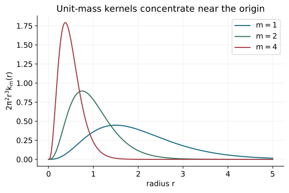
The radial integrals use ${\int }_0^{\infty }{r}^n{e}^{-2mr}dr=n!/(2m{)}^{n+1}$. Taking the ratio of the $n=5$ and $n=3$ integrals gives $5/m^2$. Isotropy distributes this equally among four coordinates, giving $5/(4m^2)$ per coordinate.

For $m=10$ in fixed inverse-length units, the mean squared radius is $0.05$. Doubling $m$ divides it by four. This quantifies localization while the normalization calculation separately fixes the delta coefficient.

What is established

The integral, moments, and distributional limit are exact. The source’s contact recovery is conditional on its geometric, determinant, and measure inputs. The missing factor cannot be silently absorbed while claiming to have independently verified the coupling.

Looking ahead

IV.7 derives the renormalization-group scale from a specified beta function, independently of whether the proposed induced construction realizes that beta function.

Figures for the calculation

Problem set

1. Classroom core. Integrate the unnormalized source kernel with ordinary $d^{4}x$.

2. Self-study calculation. Find the normalized kernel’s mean squared radius at $m=20$.

3. Self-study interpretation. Does an upper bound by an exponential determine the delta coefficient?

4. Research extension. Derive the actual two-touching kernel from the determinant.

Answer checkpoints

1. The integral is $3{\pi }^2$, independent of $m$.

2. It is $5/400=0.0125$.

3. No. It shows suppression away from the diagonal; the measure, prefactor, and total mass determine the coefficient.

4. Completion: identify the ambient measure and tensor contraction, prove convergence on test functions, and track the normalization into the proposed coupling.

Teaching note

Use the decisive step in problem 2 as the written exit check for IV.6; assign problem 3 only after students have named the assumptions. Grade the research extension by its documented method and justified conclusion, including an unresolved result when evidence is missing. The timing above awaits classroom rehearsal.

Previous note · Next note · Course guide