Mini-Lecture V.2: Twistor Parametrization of the Measure

We study the Jacobian matrix and its gauge zero mode. The worked calculation and its limitations are the classroom target; the longer source reconstruction supports independent study.

How to use this lecture

Prerequisites: III.6; Hermitian matrices and eigenvectors. Review the relevant prerequisite bridge before starting.

• Classroom core, 90 minutes: question and prerequisites (10); the Jacobian matrix and its gauge zero mode (25); worked calculation or laboratory (30); problems 1–2 (20); written exit check (5).
• Self-study, approximately 2–3 hours: reconstruct the algebra in the main text, work through the laboratory, then solve problems 1–3 before reading the answer checkpoints. The estimate is provisional.
• Research extension: problem 4 states the source-dependent task and what counts as completion. Its open claims are not assumed in the classroom assessment.

The classroom result is the explicitly calculated model or conditional derivation below. Retained sections marked Source reconstruction explain the IAS argument and identify provenance; that label does not certify the argument. The claim map records the research limits. The literal extended-surface identity fails the circle check in III.5; geometric QCD conclusions depending on it remain conditional.

Reading

• Primary: IAS lectures, pages 113-117. Consult the page images when an equation is clipped or extraction is ambiguous.
• Gentler route: the prerequisite bridges, followed by this lecture’s worked calculation.
• Optional research: the bibliography and version map identifies the primary papers for this module and their role.

Source Pages

Primary source: IASQCDLectures.pdf, pages 113-117.

The Question

How are loop velocities replaced by twistor variables?

Notation

• $v_{\alpha }(\theta )={\dot{x}}_{\alpha }$: the loop velocity.
• $f_{a^{\prime }}^{\prime }{\sigma }^{\alpha }={\lambda }_{a^{\prime }}\otimes {\mu }_{\dot{b}}$: the null twistor factorization (eq (102)).
• $v_{\alpha }=2\mathrm{Re}(iz\lambda {\sigma }_{\alpha }\mu ){|}_{z=e^{i\theta }}$: the velocity reconstructed from twistors (eq (103)).
• $\Lambda =\bar{\lambda }\lambda =\bar{\mu }\mu$: the common spinor norm (Faddeev-Popov constraint).
• $\hat{Q}$: the $4\times 4$ kernel of the twistor measure (eq (106)).
• ${\omega }_1=0,{\omega }_2=2\Lambda ,{\omega }_{3,4}=\Lambda$: the eigenvalues of $\hat{Q}$.
• $\sqrt{{\det }^{\prime }Q}=\sqrt{2{\Lambda }^3}$: the Faddeev-Popov Jacobian (eq (108)).
• $J_{\mathrm{total}}=2{\Lambda }^2$: the total measure after zero-mode elimination (eq (113)).
• $U(1)$: the residual gauge invariance.
• $S^3\times S^3/U(1)$: the coset space of normalized spinors.

Derivation

Step 1 — The phase-space measure and the Virasoro constraint (p113, eqs (101)-(103))

The phase-space measure (p113, eq (101)) is

$$\mathcal{DP}\mathcal{D}X\propto {\delta }^{(4)}\left(\int v(\theta )d\theta \right)\prod _{\theta }{d}^{4}p(\theta )d^{4}v(\theta ).$$

On a nonzero patch satisfying the conformal constraint $(f_{\mu }^{\prime }{)}^2=0$, factor the holomorphic tangent (p113, eq (102)). This is a parametrization of null vectors; reaching that constraint from arbitrary boundary labels requires the separate reparametrization problem in III.5:

$$f_{\alpha }^{\prime }{\sigma }_{a\dot{b}}^{\alpha }={\lambda }_a(z){\mu }_{\dot{b}}(z).$$

This converts the loop velocity algebraically into twistor bilinears (p113, eq (103)):

$$v_{\alpha }(\theta )=2\mathrm{Re}(iz\lambda {\sigma }_{\alpha }\mu ){|}_{z=e^{i\theta }}.$$

The source proposes to use these boundary spinor variables in the functional integral. The local factorization does not by itself establish the full measure change or its global domain.

What is being used: the Virasoro constraint (III.5) and the twistor factorization (III.6). Status: Source reconstruction.

Step 2 — The measure change: the kernel $\hat{Q}$ (p114, eqs (104)-(106))

The change of variables $v\to (\lambda ,\mu )$ induces a metric on the twistor tangent space. The norm of a variation (p114, eq (104)) is

$$\Vert \delta v{\Vert }^2=\int d\theta (\delta v_{\alpha }{)}^2\propto \int d\theta |z\delta \lambda {\sigma }_{\alpha }\mu +z\lambda {\sigma }_{\alpha }\delta \mu -c.c.{|}^2.$$

Expanding with Fierz identities, this becomes a quadratic form (p114, eq (105)):

$$\Vert \delta v{\Vert }^2\propto \int d\theta \delta {\Lambda }^{†}\cdot \hat{Q}\cdot \delta \Lambda ,$$

where $\delta \Lambda =(\delta \lambda ,\delta \mu {)}^T$ and the kernel is the $4\times 4$ block matrix (p114, eq (106)):

$$\hat{Q}=\left(\begin{array}{cc}(\bar{\mu }\mu )I_2& \lambda \bar{\mu }\\ \mu \bar{\lambda }& (\bar{\lambda }\lambda )I_2\end{array}\right).$$

What is being used: the Fierz identity and the quadratic-form structure. Status: Source reconstruction.

Step 3 — The eigenvalues and the Faddeev-Popov Jacobian (p115, eqs (107)-(108))

The eigenvalues of $\hat{Q}$ (with $\Lambda =\bar{\lambda }\lambda =\bar{\mu }\mu$ on the constraint surface) are (p115):

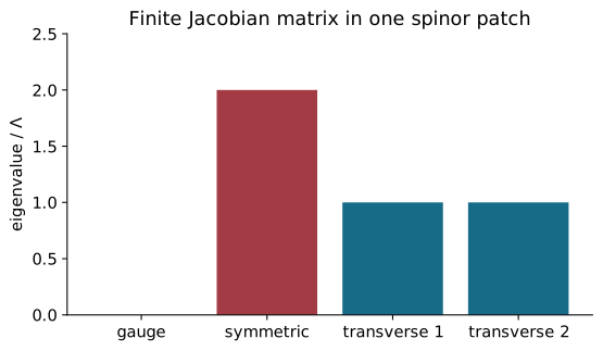
1. ${\omega }_1=0$: the zero mode (gauge transformation $\delta \lambda =\epsilon \lambda$, $\delta \mu =-\epsilon \mu$).
2. ${\omega }_2=2\Lambda$: the dilatation mode ($\delta \lambda =\lambda$, $\delta \mu =\mu$).
3. ${\omega }_{3,4}=\Lambda$: rotation modes orthogonal to the spinors.

The determinant vanishes due to the zero mode. The source identifies a Jacobian with the square root of the nonzero-eigenvalue product (p115, eq (107)). The finite matrix product is verified below; its interpretation as the full real Faddeev–Popov measure needs additional input:

$$d^{4}v(\theta )=\sqrt{\stackrel{\prime }{\det }Q}d{\Omega }_{\mathrm{FP}}(\lambda ,\mu ),$$

and evaluating the determinant on the physical subspace gives (p115, eq (108)):

$$\sqrt{\stackrel{\prime }{\det }Q}=\sqrt{2{\Lambda }^3}.$$

What is being used: the Faddeev-Popov procedure for gauge fixing. Status: standard (Faddeev-Popov); Source reconstruction (the eigenvalue computation).

Step 4 — Eliminating the zero mode (p116, eqs (109)-(113))

The zero mode is the gauge orbit $\delta \lambda =\delta r\lambda$, $\delta \mu =-\delta r\mu$ (p116, eq (109)). The norm along the gauge orbit (p116, eqs (110)-(111)) is $\Vert {\delta }_{\mathrm{gauge}}{\Vert }^2=2\Lambda (\delta r{)}^2$, giving $\sqrt{\det G_{\parallel }}=\sqrt{2\Lambda }$ (eq (112)).

The source then proposes the product (p116, eq (113)):

$$J_{\mathrm{total}}=\sqrt{\stackrel{\prime }{\det }Q}\times \sqrt{\det G_{\parallel }}=\sqrt{2{\Lambda }^3}\times \sqrt{2\Lambda }=2{\Lambda }^2.$$

Step 5 — The residual $U(1)$ and the coset $S^3\times S^3/U(1)$ (p117)

After the Faddeev-Popov fixing, a residual local $U(1)$ gauge invariance remains: $(\lambda ,\mu )\to (e^{i\phi }\lambda ,e^{-i\phi }\mu )$. This is factored out, and the normalized spinors $\xi ,\eta$ (with $\bar{\xi }\xi =\bar{\eta }\eta =1$) vary on $S^3\times S^3$. After the $U(1)$ quotient, the physical spinor space is the coset $S^3\times S^3/U(1)$ (p117).

Worked laboratory: diagonalizing the measure matrix

Choose equal normalized directions $\lambda =\mu =(\sqrt{\Lambda },0{)}^T$ with $\Lambda >0$. The displayed matrix becomes

$$Q=\Lambda \left(\begin{array}{cccc}1& 0& 1& 0\\ 0& 1& 0& 0\\ 1& 0& 1& 0\\ 0& 0& 0& 1\end{array}\right).$$

The vectors $(1,0,-1,0)$ and $(1,0,1,0)$ have eigenvalues $0$ and $2\Lambda$; $(0,1,0,0)$ and $(0,0,0,1)$ have eigenvalue $\Lambda$. Thus the product of nonzero eigenvalues is $2{\Lambda }^3$, and its square root is $\sqrt{2{\Lambda }^3}$.

This verifies the finite Hermitian matrix spectrum. It does not determine by itself the real integration measure, the division by a complex gauge orbit, or the normalization of a functional Faddeev–Popov determinant. The gauge fixing must specify which real variables and orbit metric are being integrated.

At $\Lambda =0$ all eigenvalues vanish; the nonzero-spinor coordinate patch breaks down. Such degenerate points require separate treatment rather than division by the same Jacobian.

What Was Proved, What Was Assumed

Claim	Status
The Virasoro constraint factorizes $f^{\prime }=\lambda \otimes \mu$ (eq (102))	standard (III.5-III.6)
The velocity is $v=2\mathrm{Re}(iz\lambda \sigma \mu )$ (eq (103))	Source reconstruction
The kernel $\hat{Q}$ (eq (106)) with eigenvalues $0,2\Lambda ,\Lambda ,\Lambda$	Source reconstruction
$\sqrt{{\det }^{\prime }Q}=\sqrt{2{\Lambda }^3}$ (eq (108))	Source reconstruction
$J_{\mathrm{total}}=2{\Lambda }^2$ (eq (113))	Source reconstruction
The physical spinor space is $S^3\times S^3/U(1)$	Source reconstruction

The algebraic product in this last formula is correct once its two factors are assumed. The real integration variables, orbit division, and phase quotient must be fixed before it can be used as a functional measure. A complex null direction is not a count of one real redundant coordinate.

Common Traps

• Confusing the Faddeev-Popov zero mode with a physical mode. The ${\omega }_1=0$ eigenvalue is a gauge redundancy (the real rescaling $\lambda \to e^r\lambda$, $\mu \to e^{-r}\mu$), not a physical degree of freedom. It is removed by the constraint $\bar{\lambda }\lambda =\bar{\mu }\mu$.
• Forgetting the residual $U(1)$. After the Faddeev-Popov fixing, a $U(1)$ phase rotation remains. This is not fixed by the FP procedure — it is factored out separately, giving the coset $S^3\times S^3/U(1)$.

Source Map

Subsection	Source page	Slide equations
Twistor parametrization; Virasoro; $f^{\prime }=\lambda \otimes \mu$; velocity from twistors	p113	eq (101), eq (102), eq (103)
The measure change; kernel $\hat{Q}$	p114	eq (104), eq (105), eq (106)
The local Jacobian; eigenvalues; $\sqrt{{\det }^{\prime }Q}=\sqrt{2{\Lambda }^3}$	p115	eq (107), eq (108)
Elimination of the zero mode; $J_{\mathrm{total}}=2{\Lambda }^2$	p116	eqs (109)-(113)
Summary; residual $U(1)$; $S^3\times S^3/U(1)$	p117	(prose)

Figures for the calculation

Problem set

1. Classroom core. Find the eigenvalues for $\Lambda =2$.

2. Self-study calculation. Compute the pseudodeterminant and its square root for $\Lambda =2$.

3. Self-study interpretation. Why is omitting a zero eigenvalue not the complete gauge-fixing procedure?

4. Research extension. Derive the measure in one finite spinor patch.

Answer checkpoints

1. They are $0,4,2,2$.

2. They are $16$ and $4$.

3. One must also specify the gauge condition, orbit volume or metric, residual symmetry, real-variable measure, and degenerate patches.

4. Completion: exhibit the coordinate map, gauge condition, real Jacobian, residual phase quotient, and domain. Compare its homogeneity with the source formula before taking a functional product.

Teaching note

Use the decisive step in problem 2 as the written exit check for V.2; assign problem 3 only after students have named the assumptions. Grade the research extension by its documented method and justified conclusion, including an unresolved result when evidence is missing. The timing above awaits classroom rehearsal.

Previous note · Next note · Course guide