Lecture 14 — Large N and the conditions for a semiclassical bulk

A bulk described by a few weakly coupled fields must come from a boundary theory with a large number of degrees of freedom. This lecture makes that statement precise in the form ‘t Hooft gave it: in a theory of $N\times N$ matrices, Feynman diagrams are organized by the topology of surfaces, connected correlators of single-trace operators fall as $N^{2-n}$, and the theory becomes a generalized free field at infinite $N$. We verify the counting exactly in the Gaussian matrix model, where the planar limit is the Wigner semicircle and the corrections are a genus expansion. Maldacena’s example then fixes the dictionary, $L^3/G_5=2N^2/\pi$ and $L^4/{\alpha }^{\prime 2}=\lambda$, and separates the two expansions it contains. Large $N$ controls bulk loops; a local bulk with Einstein dynamics needs in addition a large gap in the spectrum.

How to use this lecture

Classroom core, two meetings of two hours. The first meeting covers ‘t Hooft’s idea and the central-limit counterexample (§§1–2, 25 minutes), double-line counting (§3, 40 minutes), and the Gaussian matrix model as a worked example (§4, 40 minutes), leaving 15 minutes for Checkpoints 1 and 2. The second meeting covers single-trace operators and factorization (§5, 30 minutes), Maldacena’s parameter map and its two expansions (§6, 40 minutes), and the conditions beyond large $N$ (§7, 25 minutes), with 25 minutes for Problems 1–4; Problems 5 and 6 complete the core assignment. These allocations are proposals and have not been tested in class.

Self-study. The code subspace of a semiclassical description (§8) and Problems 7–12, including the genus-one count for $\mathrm{Tr}{\Phi }^6$ and the contrasting counting of vector models.

Research extension. The counting of solutions to crossing that correspond to bulk interactions, and the planar density of a matrix model with a quartic potential, in Problems 13–15.

Prerequisites. Lecture 12 for generalized free fields and double-trace families, Lecture 13 for the bulk spectrum, and Wick’s theorem. The Catalan numbers and the Euler characteristic of a surface are recalled where they enter.

What this lecture establishes. The counting of §§2–5 is exact in the models where it is carried out, and it holds diagram by diagram in perturbation theory for any matrix theory. The parameter map of §6 is exact within Maldacena’s correspondence, which is the holographic input. The statements of §7 about locality and the gap are stated results with their sources.

0. Reading

Primary.

• G. ‘t Hooft, A planar diagram theory for strong interactions, Nucl. Phys. B 72 (1974) 461.
• O. Aharony, S. S. Gubser, J. Maldacena, H. Ooguri, Y. Oz, Large N Field Theories, String Theory and Gravity (1999), Sections 1.1 and 3.1.
• J. Maldacena, The Large N Limit of Superconformal Field Theories and Supergravity (1997).

Secondary.

• S. Coleman, 1/N, in Aspects of Symmetry (Cambridge, 1985), and E. Brézin, C. Itzykson, G. Parisi, J.-B. Zuber, Planar diagrams, Commun. Math. Phys. 59 (1978) 35.
• P. Di Francesco, P. Ginsparg, J. Zinn-Justin, 2D Gravity and Random Matrices (1993), Sections 1–2: the genus expansion of matrix integrals.
• D. Harlow, TASI Lectures on the Emergence of the Bulk in AdS/CFT (2018), Section 2.4.

Optional research reading.

• I. Heemskerk, J. Penedones, J. Polchinski, J. Sully, Holography from Conformal Field Theory (2009), and S. El-Showk, K. Papadodimas, Emergent Spacetime and Holographic CFTs (2011).
• I. R. Klebanov, A. M. Polyakov, AdS Dual of the Critical O(N) Vector Model (2002).
• X. O. Camanho, J. D. Edelstein, J. Maldacena, A. Zhiboedov, Causality Constraints on Corrections to the Graviton Three-Point Coupling (2014).

1. ‘t Hooft’s idea

In 1974 ‘t Hooft looked for a small parameter in quantum chromodynamics, which has none in its coupling at low energies. He proposed to use the number of colors: replace $SU(3)$ by $SU(N)$ and expand in $1/N$, holding fixed the combination $\lambda =g^{2}N$. Drawing each gluon propagator as a pair of lines carrying color indices, he found that the diagrams are organized by the topology of the surfaces they fill in. The planar diagrams dominate, and every handle costs a factor $1/N^2$. This is the structure of a string theory whose coupling is $1/N$, and ‘t Hooft conjectured that large-$N$ QCD is a theory of free strings. At large $N$ mesons are then free, with cubic couplings of order $1/\sqrt{N}$, as ‘t Hooft’s counting implies, and Witten showed in 1979 that baryons are heavy solitons whose mass grows as $N$. Brézin, Itzykson, Parisi and Zuber solved matrix integrals exactly at large $N$ in 1978, and the planar limit turned out to be a classical problem for a continuous density of eigenvalues.

Maldacena’s correspondence is the sharpest realization of ‘t Hooft’s conjecture: the strings exist, they live in AdS${}_5\times S^5$, and their coupling is $g_s=\lambda /(4\pi N)$. This lecture asks what the large-$N$ counting supplies by itself, what the parameter map of the correspondence adds, and which further conditions a semiclassical bulk with a few fields requires. The answers are needed in Lecture 15, where the overall normalization of the bulk action controlled every correlator.

2. Gaussian behavior without gravity

Consider independent, identically distributed commuting random variables $X_a$, or commuting observables in independent copies of a quantum state, with mean zero and finite cumulants, and define

$$Y_N=\frac{1}{\sqrt{N}}\sum _{a=1}^N{X}_a.$$

Independence makes cumulants additive, so that

$${\kappa }_n(Y_N)=N^{1-n/2}{\kappa }_n(X_1).$$

The variance stays finite while every higher cumulant vanishes, and $Y_N$ becomes Gaussian: this is the central limit theorem. [Proved.] Nothing in this model resembles a bulk spacetime. Small connected correlators are therefore a consequence of having many degrees of freedom, and the task of the following sections is to identify the additional structure that matrix theories have. In the quantum version the ordering of operators must also be specified. A vanishing connected four-point function can describe a free quantum field with a nonzero commutator, which is a Gaussian quantum system; classical random variables are the special case in which all commutators vanish.

3. Double-line counting

Consider a theory of an $N\times N$ Hermitian matrix field with an action normalized as

$$S=N\int d^{d}x\mathrm{Tr}\left[\frac{1}{2}(\partial \Phi {)}^2+\frac{1}{2}{m}^2{\Phi }^2+\sum _{k\ge 3}\frac{g_k}{k}{\Phi }^k\right],$$

with the couplings $g_k$ held fixed as $N$ grows. The overall factor $N$ is ‘t Hooft’s choice: it makes every term of the action of the same order. In Feynman rules the propagator carries $1/N$,

$$⟨{\Phi }_{ij}{\Phi }_{kl}⟩\propto \frac{1}{N}{\delta }_{il}{\delta }_{jk},$$

and is drawn as a double line, one line for each index. Each vertex carries a factor $N$, and each closed index line contributes a sum ${\sum }_i{\delta }_{ii}=N$. A connected vacuum diagram with $V$ vertices, $E$ propagators and $F$ closed index loops therefore scales as

$$N^{V-E+F}.$$

The double lines thicken the diagram into a surface whose faces are the index loops, and $V-E+F$ is the Euler characteristic $\chi =2-2g$ of the closed oriented surface of genus $g$ obtained by filling them in. The free energy is thus a genus expansion,

$$\log Z=\sum _{g\ge 0}{N}^{2-2g}{F}_g(g_k),$$

where $F_g$ collects all diagrams of genus $g$. The planar diagrams, $g=0$, give the leading term of order $N^2$, and every handle costs $1/N^2$. [Proved, diagram by diagram in perturbation theory.] Resummation of the series and the existence of the limit are separate questions, answered only in special cases.

Physical picture: a genus expansion is a string perturbation series. A closed-string amplitude is a sum over worldsheets of genus $g$ weighted by $g_s^{2g-2}$. The matrix expansion has the same form with $g_s\sim 1/N$, and the faces of a planar diagram fill in a surface that plays the role of a discretized worldsheet. This is why ‘t Hooft expected strings at large $N$. The analogy is exact as a statement about the combinatorics of diagrams; whether the surfaces become a continuum worldsheet with a local string action is a dynamical question, answered affirmatively only in specific theories such as the one of §6.

4. A worked example: the Gaussian matrix model

The counting can be tested exactly in the zero-dimensional Gaussian model, a single Hermitian matrix with covariance

$$⟨{\Phi }_{ij}{\Phi }_{kl}⟩=\frac{1}{N}{\delta }_{il}{\delta }_{jk}.$$

Consider the normalized moments $⟨\frac{1}{N}\mathrm{Tr}{\Phi }^{2k}⟩$. Wick’s theorem writes each as a sum over pairings of the $2k$ matrices around the trace. A pairing contributes $N^{-k}$ from its propagators, $N^F$ from its index loops, and $N^{-1}$ from the normalization, so

$$⟨\frac{1}{N}\mathrm{Tr}{\Phi }^{2k}⟩=\sum _{\text{pairings}}{N}^{F-k-1}.$$

For $k=2$ there are three pairings (Figure 1(a)). The two that do not cross have $F=3$ index loops and contribute $N^0$ each; the crossing pairing has $F=1$ and contributes $N^{-2}$. Therefore

$$⟨\frac{1}{N}\mathrm{Tr}{\Phi }^4⟩=2+\frac{1}{N^2}.$$

The crossing pairing cannot be drawn on a sphere without crossing lines, but it can be drawn on a torus: it is the genus-one term. The same enumeration gives

$$⟨\frac{1}{N}\mathrm{Tr}{\Phi }^6⟩=5+\frac{10}{N^2},⟨\frac{1}{N}\mathrm{Tr}{\Phi }^8⟩=14+\frac{70}{N^2}+\frac{21}{N^4},$$

numbers first organized in general by Harer and Zagier. [Exact calculation.] The leading coefficients $1,2,5,14$ are the Catalan numbers $C_k=\frac{1}{k+1}\left(\genfrac{}{}{0ex}{}{2k}{k}\right)$, which count the pairings without crossings (Problem 4).

The planar limit has a simple meaning. The Catalan numbers are the moments of the Wigner semicircle,

$${\int }_{-2}^{2}dx{x}^{2k}\frac{\sqrt{4-x^2}}{2\pi }=C_k,$$

so at infinite $N$ the eigenvalues of $\Phi$ are distributed with the continuous density $\rho (x)=\sqrt{4-x^2}/(2\pi )$ on $[-2,2]$ (Figure 1(b)). The matrix has $N^2$ degrees of freedom, but its planar limit is described by one classical function, determined by a saddle point, as Brézin, Itzykson, Parisi and Zuber showed for general potentials. The corrections in $1/N^2$ are the genus expansion of §3.

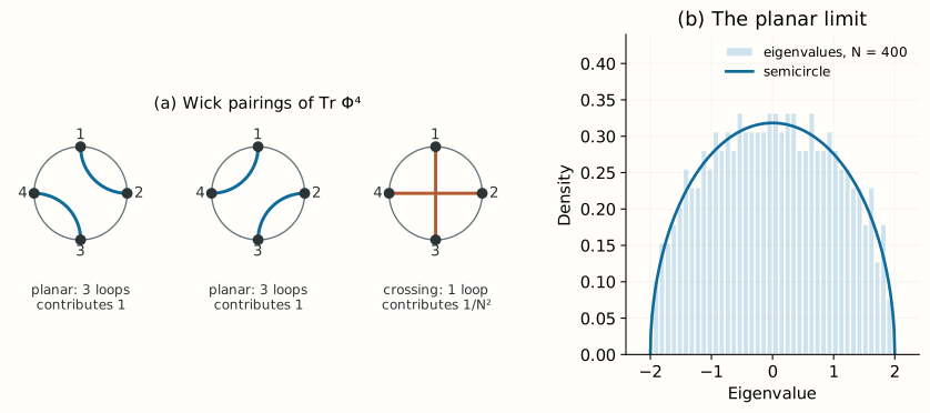
Checkpoint 1. Why does the crossing pairing in $\mathrm{Tr}{\Phi }^4$ have only one index loop?

Answer. Write the trace as ${\Phi }_{i_1{i}_2}{\Phi }_{i_2{i}_3}{\Phi }_{i_3{i}_4}{\Phi }_{i_4{i}_1}$. The non-crossing pairing $(12)(34)$ leaves $i_2$ and $i_4$ as free sums, each closing a loop inside one propagator, and identifies $i_1$ with $i_3$ in a third loop. The crossing pairing $(13)(24)$ identifies all four indices, so the four index sums collapse into one loop.

5. Single-trace operators and factorization

The operators whose correlators have a simple large-$N$ limit are the single-trace operators, such as $\mathrm{Tr}{\Phi }^k$ and their derivatives. In the Gaussian model the connected correlators of $Q=\mathrm{Tr}{\Phi }^2$ can be computed exactly. The $N^2$ real components of $\Phi$ are independent Gaussian variables of variance $1/N$, so

$$\log ⟨e^{tQ}⟩=-\frac{N^2}{2}\log \left(1-\frac{2t}{N}\right),{\kappa }_n(Q)=2^{n-1}(n-1)!N^{2-n}.$$

The mean is $N$, the variance is $2$, and the connected three- and four-point functions are $8/N$ and $48/N^2$. [Exact calculation.] This is the general pattern. For single-trace operators normalized to have connected two-point functions of order one, the connected $n$-point function is of order $N^{2-n}$, because each additional operator inserts one more boundary into the planar surface and costs one power of $N$.

Two consequences follow at infinite $N$. First, every connected correlator beyond the two-point function vanishes, so single-trace operators become generalized free fields: their correlators factorize into sums of products of two-point functions. Second, products such as $:\mathrm{Tr}{\Phi }^2\mathrm{Tr}{\Phi }^2:$ are new, independent operators, the double traces, whose dimensions at infinite $N$ are sums of single-trace dimensions. In the language of Lectures 12 and 13, single-trace operators are single particles in the bulk, double traces are two-particle states, and the connected three-point function of order $1/N$ is a cubic bulk coupling. Lecture 15 found the same structure from the bulk side: the tree-level generating functional is proportional to the normalization $\mathcal{N}{L}^{d-1}$ of the bulk action, which gives normalized $n$-point functions of order $(\mathcal{N}{L}^{d-1}{)}^{1-n/2}$. Matching the two expansions identifies $\mathcal{N}{L}^{d-1}\sim N^2$.

Checkpoint 2. In the Gaussian model, what is the connected four-point function of the normalized fluctuation $\hat{Q}=(Q-N)/\sqrt{2}$?

Answer. ${\kappa }_4(Q)/4=12/N^2$, of order $N^{2-4}$, while its variance is one.

6. Maldacena’s example and its two expansions

In the correspondence between $\mathcal{N}=4$ super-Yang–Mills theory with gauge group $SU(N)$ and type IIB string theory on AdS${}_5\times S^5$, the parameters are related by

$$g_{\mathrm{YM}}^2=4\pi g_s,\lambda =g_{\mathrm{YM}}^{2}N,L^4=4\pi g_{s}N{\alpha }^{\prime 2}=\lambda {\alpha }^{\prime 2},$$

where $L$ is the common radius of AdS${}_5$ and $S^5$ and ${\alpha }^{\prime }$ the square of the string length. Newton’s constant in ten dimensions is $G_{10}=8{\pi }^6{g}_s^2{\alpha }^{\prime 4}$, and reducing on $S^5$, of volume ${\pi }^3{L}^5$, gives the five-dimensional constant $G_5=G_{10}/({\pi }^3{L}^5)$. Therefore

$$\frac{L^3}{G_5}=\frac{2N^2}{\pi }.$$

[Exact within the correspondence.] The overall normalization of the bulk action, $L^3/G_5$, is of order $N^2$, which is the identification made at the end of §5. The stress-tensor coefficient $C_T$ of Lecture 12 is proportional to the same quantity.

The correspondence contains two independent expansions. Bulk loops are suppressed by $G_5/L^3\sim 1/N^2$, the genus expansion of §3. Stringy corrections are suppressed by ${\alpha }^{\prime }/L^2=1/\sqrt{\lambda }$, and they measure how much the strings resolve the curvature of AdS. Classical supergravity requires both parameters to be large: first $N\to \infty$ at fixed $\lambda$, which keeps the planar diagrams, and then $\lambda \to \infty$. Gubser, Klebanov and Polyakov noticed in their first paper that this has a direct consequence for the spectrum. A string state at excitation level $n$ has mass $m^2\simeq 4n/{\alpha }^{\prime }$, so the dimension of the dual operator is

$$\Delta \simeq mL=2\sqrt{n}{\lambda }^{1/4},$$

which grows without bound at strong coupling (Problem 12). At large $\lambda$ only the supergravity fields, whose dimensions stay of order one, remain light. The gap between them and the string states is what allows a description by a few fields.

7. What large N does not supply

The counting of §§3–5 holds in any theory of matrices, and a version of it holds for vectors. An $O(N)$ model of $N$ scalars ${\varphi }^a$ has single-trace operators such as ${\varphi }^a{\varphi }^a$, and its connected correlators fall as powers of $1/N$, with $C_T$ of order $N$. It has a large-$N$ limit with factorization, generalized free fields and double traces. But its spectrum of single-trace operators includes the conserved currents ${\varphi }^a{\partial }^s{\varphi }^a$ of every even spin $s$, whose dimensions $s+d-2$ grow only linearly with spin, so there is no gap. Klebanov and Polyakov proposed that the bulk dual of the singlet sector contains a massless field of every even spin, the minimal version of Vasiliev’s higher-spin gravity, which is far from Einstein gravity with a few matter fields.

Heemskerk, Penedones, Polchinski and Sully turned this into a criterion. They counted the solutions of the crossing equations at order $1/N^2$ in a theory whose only light single-trace operator is a scalar, and found that the solutions whose anomalous dimensions are supported at spins up to $L$ correspond one to one with the quartic contact interactions in AdS whose contributions stop at spin $L$. For even $L$ there are $(L+2)(L+4)/8$ of them: at $L=2$, the vertices ${\varphi }^4$ and $(\nabla \varphi {)}^4$ and one vertex with six derivatives. A large gap ${\Delta }_{\mathrm{gap}}$ to single-trace operators of spin greater than two then suppresses the higher-derivative interactions, as the stringy corrections of §6 are suppressed at large $\lambda$. [Stated only — refs: Heemskerk, Penedones, Polchinski, Sully; El-Showk, Papadodimas.] Camanho, Edelstein, Maldacena and Zhiboedov later showed that causality in the bulk forces the corrections to the graviton three-point coupling to be controlled by the same gap. A semiclassical bulk described by Einstein gravity with a few fields therefore requires two conditions: a large $C_T$, which suppresses loops, and a sparse spectrum with a large gap, which makes the bulk interactions local. Neither implies the other.

8. Self-study: why the bulk description has a code subspace

A low-energy bulk effective theory describes a restricted family of boundary states. Choose a reference semiclassical background and a set of excitations that do not change it appreciably; their span is the candidate code subspace. In a simple dimensional estimate an excitation of energy $E$ produces a small backreaction on an AdS-sized region when

$$\frac{G_{N}E}{L^{d-2}}\ll 1,\text{equivalently}EL\ll \frac{L^{d-1}}{G_N}\sim N^2.$$

This condition is necessary but not sufficient. Energy localized in a small region, large occupation numbers, the vicinity of horizons and collective effects impose stronger restrictions. The logical parallel with Lecture 7 is direct: a reconstruction map is tested on a specified family of inputs, and enlarging the family can invalidate it. A map that works for a few low-energy excitations need not work uniformly on all black-hole microstates.

The expansion need not be uniform in time either. A correction of order $1/N^2$ at fixed time can become important at a time that grows with $N$, as the recurrences of Lecture 29 illustrate, so the limits $N\to \infty$ and $t\to \infty$ must be taken in a stated order.

9. What to take away

• Proved, diagram by diagram: with the action normalized as $N\mathrm{Tr}$, connected vacuum diagrams scale as $N^{2-2g}$, and the free energy is a genus expansion with planar leading term of order $N^2$.
• Exact calculation: in the Gaussian model $⟨\frac{1}{N}\mathrm{Tr}{\Phi }^4⟩=2+N^{-2}$; the planar coefficients are Catalan numbers, the moments of the semicircle.
• Exact calculation: the cumulants of $\mathrm{Tr}{\Phi }^2$ are $2^{n-1}(n-1)!N^{2-n}$; normalized single-trace operators have connected $n$-point functions of order $N^{2-n}$ and become generalized free fields.
• Exact within the correspondence: $L^3/G_5=2N^2/\pi$ and $L^4/{\alpha }^{\prime 2}=\lambda$; bulk loops are suppressed by $1/N^2$ and stringy corrections by $1/\sqrt{\lambda }$.
• Stated with sources: a local bulk with Einstein dynamics requires, beyond large $N$, a sparse spectrum with a large gap; vector models have large $N$ without a gap.

10. Looking ahead

Lecture 15 computes the generating functional of a single-trace scalar from the bulk and finds it proportional to $\mathcal{N}{L}^{d-1}\sim N^2$, in agreement with the counting of §5. Lecture 16 uses the same large parameter in the form $c=3L/2G_3$ for two-dimensional CFTs, and Lecture 29 returns to the generalized free fields of the planar limit as operator algebras.

11. Problem set

Classroom core

1. A cumulant count. What is the connected four-point function of $Y_N$, and what does its vanishing leave unchanged?

2. Euler’s formula. Show that a connected vacuum diagram of the matrix theory scales as $N^{V-E+F}$, and that $V-E+F=2-2g$ for the surface obtained by filling in its index loops. Find $g$ for the diagram with one quartic vertex and two propagators in each of its two inequivalent contractions.

3. The three pairings. Compute the number of index loops for each pairing of $\mathrm{Tr}{\Phi }^4$ and derive $⟨\frac{1}{N}\mathrm{Tr}{\Phi }^4⟩=2+N^{-2}$.

4. Planar pairings and Catalan numbers. Show that the number of non-crossing pairings of $2k$ points on a circle satisfies $C_k={\sum }_{j=0}^{k-1}{C}_j{C}_{k-1-j}$, and verify that the semicircle moments satisfy the same recursion.

5. Cumulants of a single-trace operator. Derive the generating function of §5 and the cumulants ${\kappa }_n(Q)=2^{n-1}(n-1)!N^{2-n}$.

6. The parameter map. Derive $L^3/G_5=2N^2/\pi$ from $G_{10}=8{\pi }^6{g}_s^2{\alpha }^{\prime 4}$, $L^4=4\pi g_{s}N{\alpha }^{\prime 2}$ and the volume of $S^5$.

Self-study consolidation

7. Two expansion parameters. Can $C_T$ be large while the bulk has important higher-derivative interactions?

8. Nonuniform limits. A correction is $t/N^2$ in units $L=1$. For which times is it small, and what does this imply for late-time statements?

9. Genus one in $\mathrm{Tr}{\Phi }^6$. Among the fifteen pairings of six points, count those with $F=4$ and those with $F=2$, and recover $5+10N^{-2}$.

10. Vector models. For $N$ real scalars with $⟨{\varphi }^a{\varphi }^b⟩={\delta }^{ab}$, show that the connected $n$-point function of $\sigma =\frac{1}{\sqrt{N}}{\sum }_a({\varphi }^a{\varphi }^a-1)$ scales as $N^{1-n/2}$. Compare the expansion parameter with that of a matrix model.

11. Backreaction. Show that $G_{N}E/L^{d-2}\ll 1$ is equivalent to $EL\ll L^{d-1}/G_N$, and evaluate the bound for $\mathcal{N}=4$ super-Yang–Mills theory in terms of $N$.

12. String states. Using $m^2\simeq 4n/{\alpha }^{\prime }$ and $\Delta (\Delta -4)=m^2{L}^2$, show that $\Delta \simeq 2\sqrt{n}{\lambda }^{1/4}$ at large $\lambda$.

Research extension

13. Testing a code subspace. Specify an error criterion for a proposed semiclassical code subspace. Known: the logic of Lecture 7 and the estimates of §8. Completion: a stated family of states and observables, a norm or operational test, and an example in which the criterion fails.

14. Crossing and bulk locality. Count the solutions of crossing at order $1/N^2$ with spin at most $L$ for a single light scalar, and match them with bulk contact interactions. Known: Heemskerk, Penedones, Polchinski and Sully. Completion: the counting for $L=0$ and $L=2$, with the corresponding bulk vertices.

15. A quartic matrix model. Find the planar eigenvalue density for the potential $\frac{1}{2}{x}^2+\frac{g}{4}{x}^4$ by the saddle-point method, and check its first moments against planar diagrams. Known: Brézin, Itzykson, Parisi and Zuber. Completion: the density, its support as a function of $g$, and the second moment to first order in $g$.

12. Answer checkpoints

1. ${\kappa }_4(Y_N)={\kappa }_4(X_1)/N$. Its vanishing leaves the variance of order one unchanged, so the limit is Gaussian with a finite width.

2. Each propagator gives $1/N$, each vertex $N$ and each closed index loop $N$. Gluing a polygon into each index loop turns the ribbon graph into a closed surface with $V$ vertices, $E$ edges and $F$ faces, whose Euler characteristic is $2-2g$. For one quartic vertex with two self-contractions the planar contraction has $F=3$ and $\chi =1-2+3=2$, genus zero, while the crossing contraction has $F=1$ and $\chi =0$, genus one.

3. Label the matrices $1,2,3,4$ around the trace. The pairings $(12)(34)$ and $(14)(23)$ each leave three index loops, and $(13)(24)$ leaves one. With the factor $N^{-2}$ from the propagators and $N^{-1}$ from the normalization, the contributions are $1,1,N^{-2}$.

4. In a non-crossing pairing, the point $1$ is paired with some point $2j+2$, and the pairing splits into non-crossing pairings of the $2j$ points inside and the $2(k-1-j)$ points outside, which gives the recursion. For the semicircle, the moments satisfy the same recursion, which follows from the equation $G(z)=1/(z-G(z))$ for its resolvent.

5. The components of $\Phi$ are $N$ real diagonal entries and $N(N-1)/2$ complex off-diagonal ones, which amount to $N^2$ real Gaussian variables $x_a$ of variance $1/N$ with $Q={\sum }_a{x}_a^2$. Each gives $⟨e^{t{x}_a^2}⟩=(1-2t/N{)}^{-1/2}$. Expanding $-\frac{N^2}{2}\log (1-2t/N)={\sum }_n\frac{N^2}{2n}{\left(\frac{2t}{N}\right)}^n$ gives ${\kappa }_n=n!\cdot \frac{N^2}{2n}{\left(\frac{2}{N}\right)}^n=2^{n-1}(n-1)!N^{2-n}$.

6. $G_5=\frac{8{\pi }^6{g}_s^2{\alpha }^{\prime 4}}{{\pi }^3{L}^5}$, so $\frac{L^3}{G_5}=\frac{L^8}{8{\pi }^3{g}_s^2{\alpha }^{\prime 4}}=\frac{16{\pi }^2{g}_s^2{N}^2{\alpha }^{\prime 4}}{8{\pi }^3{g}_s^2{\alpha }^{\prime 4}}=\frac{2N^2}{\pi }$.

7. Yes. Loops can be small while ${\Delta }_{\mathrm{gap}}$ is of order one, and then the higher-derivative and higher-spin interactions are unsuppressed; vector models are the extreme example.

8. For $t\ll N^2$. A fixed-time limit does not justify extrapolation to times of order $N^2$ or larger, where the correction is of order one.

9. There are five non-crossing pairings, each with $F=4$ and contribution $N^{4-3-1}=1$, and ten crossing pairings, each with $F=2$ and contribution $N^{-2}$; the total is $15$ pairings.

10. The variables ${\varphi }^a{\varphi }^a-1$ are independent with finite cumulants, so this is the central-limit model of §2 with the $N$ vector components as copies: ${\kappa }_n(\sigma )=N^{1-n/2}{\kappa }_n({\varphi }^2)$. The expansion parameter is $1/\sqrt{N}$ per insertion, and the expansion of the free energy runs in powers of $1/N$ rather than $1/N^2$.

11. Multiply $G_{N}E/L^{d-2}\ll 1$ by $L^{d-1}/G_N$. For $\mathcal{N}=4$ super-Yang–Mills theory, $L^3/G_5=2N^2/\pi$ gives $EL\ll N^2$.

12. At large $\Delta$, ${\Delta }^2\simeq m^2{L}^2=4n{L}^2/{\alpha }^{\prime }=4n\sqrt{\lambda }$, so $\Delta \simeq 2\sqrt{n}{\lambda }^{1/4}$.

13. Guide. State the family of states, the observables to be reconstructed, the reference system, and an error measured in operator norm or by an entangled-input test as in Lecture 7. A criterion checked on one expectation value in one state does not establish uniform recovery.

14. Guide. Expand the four-point function in double-trace blocks with anomalous dimensions ${\gamma }_{n,\ell }$ supported at $\ell \le L$, and impose crossing. For $L=0$ there is a single solution, fixed for all $n$ up to one overall constant, which matches the ${\varphi }^4$ vertex. The completion is to reproduce the count of Heemskerk, Penedones, Polchinski and Sully for $L=2$ and identify the corresponding derivative vertices.

15. Guide. The saddle-point equation for the density is $\frac{1}{2}{V}^{\prime }(x)=\mathrm{P}\int dy\frac{\rho (y)}{x-y}$, whose one-cut solution is $\rho (x)=\frac{1}{2\pi }\left(1+2g{a}^2+g{x}^2\right)\sqrt{4a^2-x^2}$ with $3g{a}^4+a^2=1$. Its second moment agrees with the planar diagrams to first order in $g$.

Wiki connections. large-N factorization