Mini-Lecture I.5: The Makeenko-Migdal Equation

We study the generator insertion and finite-color splitting. The worked calculation and its limitations are the classroom target; the longer source reconstruction supports independent study.

How to use this lecture

Prerequisites: I.4; index contraction and normalized traces. Review the relevant prerequisite bridge before starting.

• Classroom core, 90 minutes: question and prerequisites (10); the generator insertion and finite-color splitting (25); worked calculation or laboratory (30); problems 1–2 (20); written exit check (5).
• Self-study, approximately 2–3 hours: reconstruct the algebra in the main text, work through the laboratory, then solve problems 1–3 before reading the answer checkpoints. The estimate is provisional.
• Research extension: problem 4 states the source-dependent task and what counts as completion. Its open claims are not assumed in the classroom assessment.

The classroom result is the explicitly calculated model or conditional derivation below. Retained sections marked Source reconstruction explain the IAS argument and identify provenance; that label does not certify the argument. The claim map records the research limits.

Reading

• Primary: IAS lectures, pages 15-18. Consult the page images when an equation is clipped or extraction is ambiguous.
• Gentler route: the prerequisite bridges, followed by this lecture’s worked calculation.
• Optional research: the bibliography and version map identifies the primary papers for this module and their role.

Source Pages

Primary source: IASQCDLectures.pdf, pages 15-18.

The question

The Yang–Mills equation becomes a relation among Wilson-loop averages after a field-space integration by parts. We derive the insertion and color splitting explicitly, distinguishing an observable before averaging from its expectation value.

Schwinger–Dyson before averaging

Let $w_C[A]=N_c^{-1}\mathrm{tr}{U}_C[A]$ and $W[C]=⟨w_C[A]⟩$. For a regulated functional integral, vanishing of an integrated total derivative gives

$$⟨\frac{\delta O[A]}{\delta A_{\nu }^a(x)}⟩=⟨O[A]\frac{\delta S}{\delta A_{\nu }^a(x)}⟩.$$

The derivative is with respect to a color component. The action variation is proportional to $(D_{\mu }{F}_{\mu \nu }{)}^a$, not the bare trace of a commutator. At this stage $O$ is an unaveraged insertion.

Use the Hermitian convention $U=\mathcal{P}{e}^{ig\int A^a{T}^{a}dx}$, $\mathrm{tr}{T}^a{T}^b={\delta }^{ab}/2$. Varying the ordered exponential gives

$$\frac{\delta U(b,a)}{\delta A_{\nu }^c(x)}=ig{\int }_a^{b}ds{\dot{C}}_{\nu }(s){\delta }^{(4)}(C(s)-x)U(b,s)T^{c}U(s,a).$$

This inserts a generator $T^c$. It does not insert the field strength; an area derivative does that, as I.4 showed.

To derive the loop equation, apply the identity to a Wilson holonomy carrying a generator at a marked point and sum the color label. The action variation supplies the covariant divergence of the curvature insertion on the left. The variation of the holonomy supplies a second generator at the contact point on the right. Regulated point splitting handles the coincident insertion.

Worked color algebra

The $SU(N_c)$ completeness identity is

$$\sum _a(T^a{)}_{ij}(T^a{)}_{kl}=\frac{1}{2}\left({\delta }_{il}{\delta }_{jk}-\frac{1}{N_c}{\delta }_{ij}{\delta }_{kl}\right).$$

Multiplying by the two transport matrices and contracting indices gives

$$\sum _a\mathrm{tr}(T^{a}U{T}^{a}V)=\frac{1}{2}\left(\mathrm{tr}U\mathrm{tr}V-\frac{1}{N_c}\mathrm{tr}(UV)\right).$$

The first term splits the trace; the second is the finite-$N_c$ subtraction. Divide by $N_c$ and multiply by $g^2$. In normalized observables this is

$$\frac{\lambda }{2}\left(w_U{w}_V-\frac{1}{N_c^2}{w}_{UV}\right),\lambda =g^2{N}_c.$$

For $U=V=1$ both sides give $(N_c^2-1)/2$ before normalization. This checks the subtraction and the factor $1/2$.

The regulated equation and source conventions

Choose the area derivative orientation so that its covariant divergence agrees with the insertion just derived. With the above generator normalization the vector equation has the structure

$${\partial }_{\mu }^x\frac{\delta W[C]}{\delta {\sigma }_{\mu \nu }(x)}=\frac{\lambda }{2}{\oint }_{C}d{y}_{\nu }{\delta }^{(4)}(x-y)\left[⟨w_{C_{xy}}{w}_{C_{yx}}⟩-\frac{1}{N_c^2}W[C]\right].$$

The area derivative at $x$ is understood with its transport and regulator, not as an ordinary derivative of a smooth scalar. Contact terms at coincident parameters require that same prescription.

The IAS slides write a leading coefficient $\lambda$ in their loop-operator convention. We denote that coefficient by ${\lambda }_{\mathrm{loop}}$ when quoting them. With the normalized insertion used above, ${\lambda }_{\mathrm{loop}}=\lambda /2$; an alternative normalization of the area operator rescales this coefficient. Subsequent source formulas are quoted in their own convention, not used to infer a finite-$N_c$ identity with an unstated factor.

Closing the hierarchy at large $N_c$

Define the full two-loop correlator $W_2(C_1,C_2)=⟨w_{C_1}{w}_{C_2}⟩$ and its connected part $W_{2,c}=W_2-W[C_1]W[C_2]$. In the usual fixed-‘t Hooft-coupling expansion, $W_{2,c}=O(N_c^{-2})$. Thus the equation closes at leading order on the product of the two single-loop averages.

The topology explains the scaling. A connected orientable ribbon surface with genus $h$ and $b$ boundaries scales as $N_c^{2-2h-b}$ before dividing each trace by $N_c$. For two normalized traces, the planar cylinder has $h=0$, $b=2$, and contributes $N_c^{-2}$. It is not a genus-one surface.

Contact geometry

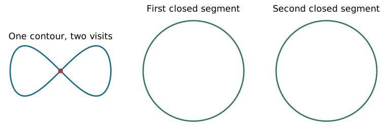
At a crossing, distinct parameters $s\ne t$ satisfy $C(s)=C(t)$. Cutting there gives closed segments $C_{st}$ and $C_{ts}$. The delta distribution expresses spacetime coincidence; the cyclic order specifies the splitting. The diagonal $s=t$ is also present and requires a regulator. A formal four-dimensional delta integrated along a one-dimensional curve cannot be treated as an ordinary finite number.

Worked laboratory: an $SU(2)$ normalization check

Choose $T^a={\sigma }_a/2$ and $U=V=1_2$. Each $\mathrm{tr}(T^a{T}^a)=1/2$, so the sum is $3/2$. The Fierz expression gives $\frac{1}{2}(2\cdot 2-\frac{1}{2}\cdot 2)=3/2$. With $g^2/N_c$ the resulting coefficient is $3g^2/4$, agreeing with $g^2{C}_F$ for $C_F=3/4$.

This check fixes a finite-color normalization. A leading planar formula quoted with a different area-operator convention must be translated before using it to assign an induced coupling.

What is established

The insertion and color algebra are exact in the regulated setting. The continuum equation is formal until its contact prescription is specified. Large-$N_c$ closure is the leading topological expansion under the usual fixed-coupling assumptions.

Looking ahead

I.6 checks the first perturbative term. I.7 examines why the singular contact structure needs more than a naive contour-dependent counterterm.

Figures for the calculation

Problem set

1. Classroom core. Evaluate ${\sum }_a\mathrm{tr}(T^a{T}^a)$ for $SU(2)$.

2. Self-study calculation. Derive the normalized split expression from the Fierz identity.

3. Self-study interpretation. Distinguish $W_2$ from $W_{2,c}$.

4. Research extension. Compare the original MM paper with IAS equation (22).

Answer checkpoints

1. Three terms of $1/2$ give $3/2$.

2. Replace each trace by $N_{c}w$ in $g^2(2N_c{)}^{-1}(\mathrm{tr}U\mathrm{tr}V-N_c^{-1}\mathrm{tr}UV)$ to obtain $(\lambda /2)(w_U{w}_V-N_c^{-2}{w}_{UV})$.

3. $W_2(C_1,C_2)=⟨w_1{w}_2⟩$ is the full correlator; $W_{2,c}(C_1,C_2)=W_2(C_1,C_2)-W[C_1]W[C_2]$ is its connected part. Only the latter is suppressed by $N_c^{-2}$.

4. Completion: record generator, action, area-derivative, and coupling conventions; translate the leading coefficient and the finite-$N_c$ subtraction. Do not compare coefficients without that dictionary.

Teaching note

Use the decisive step in problem 2 as the written exit check for I.5; assign problem 3 only after students have named the assumptions. Grade the research extension by its documented method and justified conclusion, including an unresolved result when evidence is missing. The timing above awaits classroom rehearsal.

Previous note · Next note · Course guide

Wiki connections. Wilson loop · large-N factorization