Mini-Lecture V.5: Minkowski Continuation and Helicoids

We study a real rotating surface and the scope of analytic continuation. The worked calculation and its limitations are the classroom target; the longer source reconstruction supports independent study.

How to use this lecture

Prerequisites: V.4; induced metrics and Lorentzian signature. Review the relevant prerequisite bridge before starting.

• Classroom core, 90 minutes: question and prerequisites (10); a real rotating surface and the scope of analytic continuation (25); worked calculation or laboratory (30); problems 1–2 (20); written exit check (5).
• Self-study, approximately 2–3 hours: reconstruct the algebra in the main text, work through the laboratory, then solve problems 1–3 before reading the answer checkpoints. The estimate is provisional.
• Research extension: problem 4 states the source-dependent task and what counts as completion. Its open claims are not assumed in the classroom assessment.

The classroom result is the explicitly calculated model or conditional derivation below. Retained sections marked Source reconstruction explain the IAS argument and identify provenance; that label does not certify the argument. The claim map records the research limits. The literal extended-surface identity fails the circle check in III.5; geometric QCD conclusions depending on it remain conditional.

Reading

• Primary: IAS lectures, pages 125-127. Consult the page images when an equation is clipped or extraction is ambiguous.
• Gentler route: the prerequisite bridges, followed by this lecture’s worked calculation.
• Optional research: the bibliography and version map identifies the primary papers for this module and their role.

Source Pages

Primary source: IASQCDLectures.pdf, pages 125-127.

The Question

Why move to Minkowski space before extracting masses?

Notation

• Euclidean vs. Minkowski: the signature change $(-,-,-,-)\to (+,-,-,-)$ (or $(-,+,+,+)$).
• $S_{\mathrm{Euclidean}}\to i{S}_{\mathrm{Minkowski}}$: the Euclidean action becomes $i$ times the Minkowski action.
• ${\hat{P}}_J^A$: the Fourier-projected amplitude at fixed spin $J$ (eq (132)).
• $\alpha =4\pi a$: the twist angle / Fourier projection variable.
• $M(\alpha )$: the $SU(2)$ rotation (monodromy) matrix (eq (133)).
• $dX=\phi {\phi }^{†}d\xi +\psi {\psi }^{†}d\eta$: the additive spinor parametrization (eq (134)).
• $\phi (\xi ),\psi (\eta )$: the complex eigenvectors of $SU(2)$ (eq (135)).
• $\xi =\tau +\theta$, $\eta =\tau -\theta$: left- and right-moving light-cone variables.
• $a$: the branch-point degree (controlling the twist rate).
• $R$: the radius of the rotating string.

Derivation

Step 1 — The Euclidean obstruction (p125)

The source seeks a Lorentzian interpretation of complex twistor saddles. An ordinary Euclidean factor $e^{-S_E}$ with real positive action is damped, not generically oscillatory. Complexified variables and Fourier phases can require complex saddle contours, but this is a property of the particular representation.

Complex saddles do not by themselves invalidate a theory, and real Euclidean action alone does not prove reflection positivity. Analytic continuation, the operator domain, and positivity have to be checked separately.

Step 2 — The Minkowski resolution (p125)

A Lorentzian description can make rotating classical configurations explicit. The phase is $e^{iS}$, and a real saddle is a classical stationary history. Reality of that history alone does not prove $M^2\ge 0$, a positive Hilbert space, or a real complete spectrum. The allowed spin range also requires its representation-theoretic and boundary conditions.

We use the subsequent helicoid calculation as an exact classical example. Its identification with the quantum spectrum is a conditional source proposal.

Step 3 — Twisted boundary conditions and the Fourier projection (p126, eqs (132)-(133))

To extract the spin-$J$ spectrum, project the amplitude onto fixed $J$ by a Fourier integral (p126, eq (132)):

$${\hat{P}}_J^A=\int d\alpha \exp (-ik\alpha J)A_k(\alpha ),$$

where $A_k(\alpha )$ is the amplitude after $k$ windings around the quark loop, with the rotation angle $\alpha$ introduced at every full circle. When the boundary rotates by $\alpha$, the twistors twist, and the coordinate differential transforms (p126, eq (133)):

$$d\hat{X}\to M(\alpha )d\hat{X}{M}^{†}(\alpha ),$$

where $M(\alpha )$ is an $SU(2)$ rotation matrix. This is the twisted boundary condition: the string is not periodic but twisted — after one full rotation, the coordinates are rotated by $M(\alpha )$.

Step 4 — The additive spinor parametrization (p127, eqs (134)-(135))

In Minkowski space ${\mathbb{R}}^{1,3}$, the target-space coordinate differential is parametrized by an additive sum of two independent spinor contributions (p127, eq (134)):

$$dX=\phi (\xi ){\phi }^{†}(\xi )d\xi +\psi (\eta ){\psi }^{†}(\eta )d\eta ,\xi =\tau +\theta ,\eta =\tau -\theta ,$$

where $\xi ,\eta$ are the left- and right-moving light-cone variables. The component spinors $\phi ,\psi$ are defined as complex eigenvectors of the $SU(2)$ rotation (p127, eq (135)):

$$\phi (\xi )=\sqrt{\frac{R}{2}}\left(\begin{array}{c}{e}^{i(a\xi +\pi /4)}\\ e^{-i(a\xi +\pi /4)}\end{array}\right),\psi (\eta )=\sqrt{\frac{R}{2}}\left(\begin{array}{c}{e}^{i(a\eta -\pi /4)}\\ e^{-i(a\eta -\pi /4)}\end{array}\right).$$

The parameter $a$ is the branch-point degree — it controls the rate of twisting. The $\pi /4$ phase is a convention ensuring the correct light-cone structure.

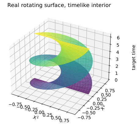
Worked laboratory: a rotating ruled surface

In Minkowski signature $(+---)$ let

$$X(\tau ,s)=(\tau ,s\cos \omega \tau ,s\sin \omega \tau ,0).$$

The tangent vectors give

$$g_{\tau \tau }=1-{\omega }^2{s}^2,g_{ss}=-1,g_{\tau s}=0.$$

The worldsheet is timelike for $|\omega s|<1$. Its endpoints become null at $|s|=1/\omega$. Put $s=\sin (\omega u)/\omega$, so $ds=\cos (\omega u)du$. Then

$$d{s}_{\mathrm{ws}}^2={\cos }^2(\omega u)(d{\tau }^2-d{u}^2).$$

The embedding solves the wave equation in these conformal coordinates: the second derivatives of the sine and cosine factors cancel between $\tau$ and $u$. Together with the conformal constraints this gives a classical Nambu–Goto surface away from the null endpoints.

This is an explicit real geometric example. It neither proves positivity of a quantum Hilbert space nor excludes negative mass-squared fluctuations around a general saddle.

What Was Proved, What Was Assumed

Claim	Status
Complex saddles in the source representation	Source-specific; not a generic obstruction to Euclidean spectral theory
Real classical rotating surface	Exact example; spectral positivity and stability need separate analysis
The Fourier projection (eq (132)) onto fixed $J$ with twist angle $\alpha =4\pi a$	Source reconstruction
The twisted boundary condition $d\hat{X}\to Md\hat{X}{M}^{†}$ (eq (133))	Source reconstruction
The additive spinor parametrization (eqs (134)-(135))	Source reconstruction

Common Traps

• Thinking the Minkowski continuation changes the theory. Equivalence requires justified analytic continuation and compatible domains. It is not proved merely by replacing a damping factor with an oscillatory one.
• Reading “twisted boundary conditions” as a gauge choice. The twist is a physical condition: the string is rotating, and after one full turn the coordinates are rotated by $M(\alpha )$. This is not a gauge redundancy — it is the encoding of the angular momentum $J$.

Source Map

Subsection	Source page	Slide equations
Source claims about continuation; qualified in this revision	p125	(prose)
Twisted boundaries; Fourier projection; $SU(2)$ monodromy	p126	eq (132), eq (133)
Additive spinor parametrization; complex eigenvectors	p127	eq (134), eq (135)

Figures for the calculation

Problem set

1. Classroom core. Find the timelike interval when $\omega =2$.

2. Self-study calculation. Derive the vanishing cross term $g_{\tau s}$.

3. Self-study interpretation. Does a real classical action prove a stable quantum spectrum?

4. Research extension. Calculate fluctuations around the displayed surface with massive endpoints.

Answer checkpoints

1. $|s|<1/2$.

2. The spatial dot product is $-\omega s\sin (\omega \tau )\cos (\omega \tau )+\omega s\cos (\omega \tau )\sin (\omega \tau )=0$.

3. No. The fluctuation operator, boundary domain, integration cycle, and positivity properties must still be analyzed.

4. Completion: specify endpoint conditions and the quadratic operator, identify its zero modes, and distinguish classical stability evidence from a complete spectral theorem.

Teaching note

Use the decisive step in problem 2 as the written exit check for V.5; assign problem 3 only after students have named the assumptions. Grade the research extension by its documented method and justified conclusion, including an unresolved result when evidence is missing. The timing above awaits classroom rehearsal.

Previous note · Next note · Course guide