Week 8 — One Head, and a Decoder Computed by Hand

Notes for the neural-networks course, Unit 2. Written by an AI assistant under the researcher’s supervision; see ai-authorship.

This is the meeting where the machine is assembled with nothing left implicit, and then run by hand on a two-token sequence until a conditional probability falls out. Everything later in the course refers back to that calculation. If it has not been done at the board, the remaining weeks rest on a component the student has never seen work.

---

Learning goals

1. Write down a complete decoder with every component fixed, and state the shape of each object.
2. Distinguish the two softmax operations by the index their probability runs over.
3. Compute a forward pass by hand, from token labels to a next-token probability and its loss.
4. Say what layer normalization constrains, and what the residual sum then does to that constraint.

Reading

Primary text. Chapter 3, §3.3 and §3.4, including the complete decoder equations of §3.4.1 and the hand calculation of §3.4.2.

Primary literature, through the bibliography: Vaswani and collaborators (2017); Ba, Kiros and Hinton for layer normalization; He and collaborators for residual connections.

Prerequisites. Week 7. Week 6 for the operation the head generalizes.

The objects and their dimensions

Let $T$ be the number of supplied positions, $d$ the representation dimension, $v$ the vocabulary size, and $L$ the number of blocks. A matrix is just a rectangular table of numbers; its shape records its number of rows and columns. Throughout this page each row represents one position. Multiplying an $a\times b$ matrix by a $b\times c$ matrix produces an $a\times c$ matrix.

Object	Shape	Meaning
$H$	$T\times d$	One vector per supplied position
$W_Q,W_K$	$d\times d_k$	Learned maps to comparison coordinates
$W_V$	$d\times d_v$	Learned map to retrieved coordinates
$Q,K$	$T\times d_k$	Query and key at each position
$V$	$T\times d_v$	Value at each position; $V$ here is not the vocabulary
$S,A$	$T\times T$	Scores and attention weights between positions
$AV$	$T\times d_v$	Retrieved vector at each position
$Z$	$T\times v$	Scores for possible next-token labels

Each symbol below has a job in this table. nn-llm-start-here previews the same computation with two positions and two components.

1. One head

One attention head begins with three learned projections of its input:

$$Q=H{W}_Q,K=H{W}_K,V=H{W}_V.$$

A learned projection here means matrix multiplication with adjustable coefficients; it need not be an orthogonal projection. Queries specify the comparison a position makes, keys supply the objects compared, and values supply the vectors that will be averaged. The projections let those three jobs use different combinations of the input coordinates, which is the whole reason there are three of them rather than one.

For an autoregressive model, position $i$ predicts the token at $i+1$ and may use $x_i$ and earlier but not $x_{i+1}$. The causal mask enforces exactly that: the score matrix is computed, entries above the diagonal are removed, and the softmax normalizes over the accessible prefix. Every row of the resulting matrix is a probability distribution. Precisely,

$$S_{ts}=\frac{q_t\cdot k_s}{\sqrt{d_k}},A_{ts}=\{\begin{array}{ll}\frac{e^{S_{ts}}}{{\sum }_{j\le t}{e}^{S_{tj}}},& s\le t,\\ 0,& s>t,\end{array}{o}_t=\sum _{s\le t}{A}_{ts}{v}_s.$$

The restriction can be implemented mathematically by replacing forbidden scores with $-\infty$ before softmax. Every row has at least its diagonal entry available. The output is $O=AV$. When rotary positions are used, rotate queries and keys as in Week 7 before computing these scores.

Physical picture. Two softmaxes appear in this architecture and they run over different index sets. The attention softmax produces a distribution over positions — over sites, in the language of a lattice model — and it answers “whom does this position consult”. The readout softmax at the end produces a distribution over token labels — over the states available at a site — and it answers “what comes next”. To interpret either distribution, first identify the index over which its probabilities sum to one.

Why divide the scores by $\sqrt{d_k}$? If query and key coordinates were independent, centred and of unit variance, their dot product would be a sum of $d_k$ independent products, hence of variance $d_k$ and typical size $\sqrt{d_k}$. Scores growing with the dimension would drive the softmax toward a single position before anything had been learned, and the division returns the variance to one.

Physical picture. Read that through Week 6 and it sharpens. The softmax over positions is a Boltzmann average with the negative scores as effective energies, so a score scale growing like $\sqrt{d_k}$ is an inverse temperature growing like $\sqrt{d_k}$ — the average would be frozen onto its lowest-energy site at initialization, with vanishing gradient to move it. The $1/\sqrt{d_k}$ is a choice of temperature scale that keeps the average soft enough to respond. It is an initialization argument, not a measured temperature, and learned queries and keys need not satisfy the independence it assumes.

Several heads run the same construction with different projections and their outputs are joined side by side (concatenated) and projected back:

$$\mathrm{MHA}(H)=[O^{(1)}\cdots O^{(h)}]W_O,W_O\in {\mathbb{R}}^{h{d}_v\times d}.$$

Here $h$ is the number of heads. Concatenation preserves each head’s retrieved coordinates until the learned output map combines them. A head is not assigned a grammatical function by this definition; any such function would have to be learned and then demonstrated.

Attention moves information between positions. The feed-forward sublayer transforms coordinates at each position separately, and it is the multilayer-neuron construction of Week 3 applied with the same parameters everywhere along the sequence.

2. Residual updates and normalization

A layer need not replace its input. A residual connection adds a computed change, so setting the change to zero preserves the input, and derivatives acquire an identity contribution: for $H^{\prime }=H+F(H)$, $J=I+J_F$. This can help propagate gradients, but does not guarantee that they remain large or small; $J_F$ can reinforce or cancel directions.

Layer normalization rescales the coordinates of one token using that token’s own mean and variance. For a row $h\in {\mathbb{R}}^d$,

$$\mu (h)=\frac{1}{d}\sum _j{h}_j,v(h)=\frac{1}{d}\sum _j(h_j-\mu {)}^2,\mathrm{LN}(h{)}_j={\gamma }_j\frac{h_j-\mu }{\sqrt{v+ϵ}}+b_j.$$

The positive $ϵ$ avoids division by zero; ${\gamma }_j,b_j$ are learned. The averaging is over the components of one position, not over sentences. Before the learned gain and shift, and with the regulator set to zero, the normalized vector has zero coordinate sum and squared norm $d$: it lies on a sphere inside the mean-zero hyperplane. With a positive regulator the squared norm is smaller, and with learned gains and shifts the geometry changes again.

The residual sum need not stay there. With $h=(1,3)$, unit gain, zero shift and $ϵ=0$, $\mu =2,v=1$, hence $\mathrm{LN}(h)=(-1,1)$. The illustrative residual map $h\mapsto h+\mathrm{LN}(h)$ gives $(0,4)$, of norm $4$ and nonzero mean. A general sublayer need not be the identity map used in this small example, so its output is still less constrained by the normalization.

Physical picture. With unit gains, zero shifts and zero regulator, normalization constrains its output to a sphere in the mean-zero hyperplane, provided the input variance is nonzero. This resembles the constraint in a spherical spin model. The residual state is the original vector plus the sublayer output, so it need not obey that constraint. Week 11 explicitly imposes unit norm on each vector and derives the resulting dynamics. Its sphere geometry is an assumption of that model.

3. The decoder, complete

Choose pre-normalization: each sublayer receives a normalized input and its output is added to the unnormalized residual state. Initialize $H^0$ by selecting the token embedding rows. Add position vectors here if using absolute positions; with the rotary convention apply the rotations inside attention instead. For blocks $\ell =0,\dots ,L-1$, define

$$U^{\ell }=H^{\ell }+{\mathrm{MHA}}_{\ell }({\mathrm{LN}}_{\ell ,1}(H^{\ell })),$$ $$H^{\ell +1}=U^{\ell }+{\mathrm{FF}}_{\ell }({\mathrm{LN}}_{\ell ,2}(U^{\ell })).$$

The feed-forward map acts on each row independently with the same parameters at every position. One concrete convention is

$$\mathrm{FF}(h)=\mathrm{ReLU}(h{W}_1+b_1)W_2+b_2,$$

where $W_1$ is $d\times m$, $W_2$ is $m\times d$, and $\mathrm{ReLU}(a)=\max (0,a)$ is applied to each component. The hidden width $m$ is a design choice. This is the hidden-layer map of Week 3 in row notation. Attention mixes positions; this sublayer transforms the coordinates within each position.

Finally set

$$Z={\mathrm{LN}}_f(H^L)W_{\mathrm{out}}+b_{\mathrm{out}},W_{\mathrm{out}}\in {\mathbb{R}}^{d\times v},p(x_{t+1}=a\mid x_{\le t})=\frac{e^{Z_{ta}}}{{\sum }_{b=1}^v{e}^{Z_{tb}}}.$$

Each bias row is added to every position. The adjustable parameters are the embedding table, all head and feed-forward matrices, normalization gains and shifts, and the output map. These equations specify a decoder convention; other nonlinearities and normalization placements define related models.

A residual block is identity plus a correction. The correction may be large. Only an additional small-step scaling, examined in Week 9, permits a controlled differential-equation interpretation.

4. The forward pass by hand

Strip the block to its bones — no normalization, no rotations, no feed-forward — and keep causal attention, a residual connection and the readout. Use the two-token context $AB$ with the two basis vectors as representations and identity projections. The matrices are

$$H=Q=K=V=I_2,S_{\mathrm{causal}}=\left(\begin{array}{cc}1/\sqrt{2}& -\infty \\ 0& 1/\sqrt{2}\end{array}\right).$$

The unmasked score matrix is $I/\sqrt{2}$; position 1 has only itself accessible, so its attention weight is one; at position 2 both are accessible and the weight on position 1 is

$$w=\frac{1}{1+e^{1/\sqrt{2}}}\simeq \mathrm{0.330238.}$$

The attention weights and the residual output are

$$A=\left(\begin{array}{cc}1& 0\\ w& 1-w\end{array}\right),H^{\prime }=H+AV=\left(\begin{array}{cc}2& 0\\ w& 2-w\end{array}\right).$$

Adding the residual gives the second token the vector $(w,2-w)$, and with a two-label identity readout,

$$p(B\mid AB)=\frac{1}{1+e^{-2(1-w)}}\simeq 0.792412,$$

whose loss is about $0.232674$ nats. Arbitrary parameters have produced a conditional probability; nothing has been trained.

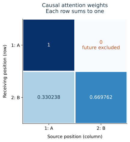
Rows are receiving positions and columns are consulted positions. The zero in the upper-right corner prevents the first representation from depending on the second token. The final vocabulary probabilities are a different normalization and are not entries of this matrix.

The intervention that follows isolates the roles of keys and values. Change the first value to zero while keeping its key fixed: the attention weights are unchanged, and the retrieved vector changes. That separates deciding where to attend from deciding what is retrieved — two jobs that the projections keep distinct even though a common input couples them.

Physical picture. That intervention is a controlled perturbation in the ordinary experimental sense, and it is worth naming because the rest of the unit’s laboratory is built from interventions of exactly this shape. One component is changed, everything else is held, and a quantity is measured before and after. What makes it informative here is that the two components are causally separated within the layer: the key determines the weight and the value determines what the weight multiplies, so moving one while holding the other isolates a mechanism rather than merely perturbing an output. In a trained network the projections share an input and the separation is no longer clean, which is precisely why the clean case is done first, by hand, where the answer is known.

Checkpoints with answers

1. For $T=4,d=6,d_k=2,d_v=3$, what are the shapes of $Q{K}^{\mathsf{T}}$ and $AV$? They are $4\times 4$ and $4\times 3$. The comparison matrix relates positions; the output retains the value dimension.

2. Remove the residual from the two-token example. What is the prediction? The last row becomes $(w,1-w)$, so $p(B)=1/[1+e^{2w-1}]\simeq 0.584075$. The change to $0.792412$ with the residual is a computed contribution, not an assumed small perturbation.

3. Set only the first value to zero, keeping queries and keys fixed. What changes? Attention stays $A$. The last residual row becomes $(0,2-w)$; its vocabulary probabilities change. A weight alone does not specify the information transmitted.

---

Subtleties and fine print

The attention softmax is over positions. It is not a distribution over possible next tokens, and a low-entropy attention row says something about which positions are consulted, not about how confident the model is in its prediction. Only the readout softmax concerns the vocabulary.

Layer normalization averages over coordinates of one vector. Not over sentences in a batch. The distinction matters as soon as a claim is made about what a normalization does to a distribution over data.

The sphere is entered and left within a single block. Normalization constrains its output; the residual sum does not. Any argument that treats hidden states as unit vectors is making an idealization, and should say so.

The $\sqrt{d_k}$ argument assumes independence at initialization. Learned queries and keys need not satisfy it, and their norms and correlations change the concentration of attention in ways the scaling does not control.

The convention is a choice. Other normalization placements and other nonlinearities exist. The equations of §3.4.1 define this course’s decoder, and a statement proved about it is a statement about that convention.

---

Key claims and status

Claim	Status
Every masked attention row is a probability distribution over accessible positions	[Exact.]
Dot-product variance $d_k$ under independent unit-variance coordinates	[Exact] under that assumption; an initialization argument
Before gain and shift, a normalized vector has zero sum and squared norm $d$	[Exact] at zero regulator
A residual sum need not remain on that sphere	[Exact], by the two-number example
$w\simeq 0.330238$, $p(B\mid AB)\simeq 0.792412$, loss $\simeq 0.232674$	[Computed] inline, every step
Changing a value with its key fixed leaves the attention weights unchanged	[Exact.]
Without a nonlinearity the feed-forward matrices collapse to one affine map	[Exact.]

---

What the week establishes

1. A complete decoder in one fixed convention, with every component and every shape stated.
2. The two softmaxes run over different index sets — positions and token labels — and the distinction is structural, not a matter of emphasis.
3. A forward pass evaluated by hand from labels to a conditional probability and its loss, with numbers the student can reproduce.
4. Layer normalization constrains its output to a sphere in the mean-zero hyperplane, and the residual sum leaves it.

What to carry forward. The hand calculation is the anchor for the rest of the course: Week 9’s indices, Week 10’s gradients and Week 11’s observables are all statements about the object computed here. When a later claim about a transformer seems too strong, the first move is to ask what it would say about this two-token example, where everything is visible.

The practical session — Laboratory 4, part I

Varied: nothing, on the first pass. The session begins with prediction. Held fixed: the provided decoder, its weights, and a short input sequence. Measured: the shape of every intermediate array — score matrix, attention weights after masking, value vectors, vocabulary scores — predicted before running and then checked; the row sums of the masked attention matrix; and what happens at a position that should not have been reachable when the mask is removed.

Product: predicted and observed dimensions side by side with every discrepancy explained; confirmation that masked rows sum to one; and a separate record of what the residual branch and the normalization each contribute to one token’s vector.

Begin by reproducing §3.4.2 by hand. A laboratory that cannot recover $0.792412$ on the two-token example should not be trusted on a trained model.

---

Connections to other parts of the wiki

• Week 7 supplies the representations and the positional information this layer consumes.
• Week 6 supplies the special case — values equal to keys — in which this head is exactly a memory update with a provable descent property.
• Week 9 asks what happens when the block of §3 is iterated, and along which index.
• Week 11 idealizes the vectors of §2 as living on a sphere; the example there is the reason that is an idealization.
• nn-llm-unit-2 — the block skeleton this note implements.

---

Start here · All weeks · Book and experiments · Previous week · Next week