Start here — How a language model makes one prediction

How a language model makes one prediction

A language model receives some text and assigns probabilities to what may come next. This course explains how a large language model (LLM) constructs those probabilities and how observations change its adjustable parameters. We start with probability, vectors and derivatives familiar to a physicist. No computer science or programming is assumed.

The wiki is a reading route in its own right. Its essential calculations are on the pages; the book and experiments offer longer arguments and ways to investigate them. The semester order is in nn-llm-week-map, and terminology can be looked up in nn-llm-glossary.

The task before the architecture

A token is one unit into which we divide text: it may be a character, a word, or part of a word. A vocabulary is the finite set of allowed tokens. The context is the sequence already supplied. If our vocabulary consists of only $A$ and $B$, the context $AB$ asks for two numbers:

$$p(A\mid AB),p(B\mid AB),p(A\mid AB)+p(B\mid AB)=1.$$

The model does not have to select a token yet. Assigning probabilities and selecting an outcome are different operations. If an observed continuation is $B$, we can judge the prediction by $-\log p(B\mid AB)$: assigning a larger probability to the observation gives a smaller loss. Week 1 derives this criterion from likelihood.

A complete small calculation

This deliberately small predictor contains one attention head and a residual sum. It omits position vectors, normalization and the feed-forward sublayer, which Week 8 will add. It is a calculable example, not a trained LLM or a claim about human language.

1. Represent the supplied tokens. Assign two numerical components to each: $A\mapsto (1,0)$ and $B\mapsto (0,1)$. Put one token in each row of a matrix:

$$H=\left(\begin{array}{cc}1& 0\\ 0& 1\end{array}\right).$$

An actual model learns such vectors. Their components are coordinates of a representation, not probabilities and not necessarily named physical observables.

2. Compare the tokens. For this example use the same vectors as queries, keys and values: $Q=K=V=H$. A query is the vector used to ask which previous positions matter; a key is the vector it is compared with; a value is the vector that will be averaged. The comparison matrix is $S=Q{K}^{\mathsf{T}}/\sqrt{2}$. Row $t$ belongs to the position being updated and column $s$ to a possible source position. The first position may not use the second, since it would then see its future. The causal restriction gives

$$S_{\mathrm{causal}}=\left(\begin{array}{cc}1/\sqrt{2}& -\infty \\ 0& 1/\sqrt{2}\end{array}\right).$$

3. Turn comparisons into weights. In each row exponentiate the allowed scores and divide by their sum. This operation is called softmax. Since $e^{-\infty }=0$, the forbidden entry gets zero weight:

$$A_{\mathrm{att}}=\left(\begin{array}{cc}1& 0\\ a& 1-a\end{array}\right),a=\frac{1}{1+e^{1/\sqrt{2}}}\simeq \mathrm{0.330238.}$$

The second position therefore receives the weighted average $a(1,0)+(1-a)(0,1)=(a,1-a)$. This is the mechanism of attention: weights computed from the current context determine which vectors are mixed.

4. Add the received information to the original vector. A residual connection means this ordinary addition:

$$H^{\prime }=H+A_{\mathrm{att}}V=\left(\begin{array}{cc}2& 0\\ a& 2-a\end{array}\right).$$

For the current context, read the last row. It contains both the original representation at that position and the contribution received by attention. The correction need not be small.

5. Produce a probability for each possible next token. Choose the identity readout, so that the two components of the last row are the scores $z_A=a$ and $z_B=2-a$. Softmax over the vocabulary now gives

$$p(B\mid AB)=\frac{e^{2-a}}{e^a+e^{2-a}}=\frac{1}{1+e^{2a-2}}\simeq \mathrm{0.792412.}$$

There were two normalizations: attention normalized over source positions; the output normalized over candidate tokens. These are different sets, although both happen to have two elements here. If the observed next token is $B$, the loss is $-\log 0.792412\simeq 0.232674$ nats.

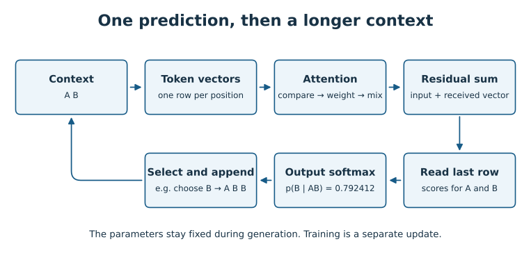
The diagram follows the same calculation. The last arrow starts a new prediction with a longer context; it is not a parameter update.

What changes in a full decoder?

Instead of our fixed identity maps, a decoder learns the token vectors, the query/key/value projections and the final readout. It also learns a nonlinear map applied separately to each position. Position information, normalization, multiple heads and repeated blocks make this construction more expressive and trainable. Week 7 introduces the representations and Week 8 assembles the block.

Training holds the observed examples fixed during an update and adjusts parameters to lower their average loss. Generation holds the parameters fixed and appends a selected token to the context. A layer changes the representation while processing one supplied sequence. Recurrence repeats a map on an internal state. Week 9 separates these four indices with a calculation.

A route through the physics

Question	Where it is answered
Why predict probabilities and minimize a logarithmic loss?	Week 1
What does context contribute?	Week 2
What is a neuron, and how can derivatives train it?	Week 3
How many constraints can weights satisfy?	Week 4
How does a fixed interaction retrieve a stored pattern?	Week 5
How does a weighted memory average lead to attention?	Week 6
How are these pieces assembled into a language model?	Weeks 7–8
How do processing, training and generation differ?	Weeks 9–10
What can physical models and measurements then explain?	Weeks 11–15

For an initial overview, read this page and the worked calculations in Weeks 1, 3, 6, 7 and 8. Return to the semester order for the complete arguments. Cover, Gardner and Hopfield retain their place in that order; this overview does not reassign lecture hours.

Check your understanding

Question. If $B$ is selected, do the parameters change?

Answer. No. The context becomes $ABB$ and the same parameters process it. Parameters change only when a training procedure uses an observed target and its loss to compute an update.

Question. Does the number $0.792412$ mean that the model is correct about language?

Answer. It is the exact consequence, to the displayed precision, of our chosen vectors and maps. Accuracy requires testing predictions against fresh observations from a specified source. Nothing was learned in this example.

Next: week-01-inferring-a-distribution. Authorship and supervision: ai-authorship.