Week 14 — Diffusion, the reverse equation, and when thermodynamics applies

Week 14 — Diffusion, reversal and thermodynamics

A decoder generates a sequence by selecting one token at a time. A diffusion model uses another construction: corrupt a complete observation with known noise, then learn a sequence of reverse transitions that can generate a new observation from noise. We will see why adding noise is easy and why reversing it requires knowledge of the data distribution.

Course: nn-llm-syllabus. Authorship and supervision: ai-authorship.

Learning goals and reading route

Compute a noisy observation at any level, distinguish a conditional from a marginal distribution, derive the noise-prediction target and its relation to the score, and check a reverse equation on a Gaussian example.

The two-hour lecture follows §§1–2, 4–6 below. Section 3, containing the posterior and variational bound, is independent study, as in Chapter 5 of the companion notes. The thermal work identity in §6 provides a specified comparison; it is not an extra assumption about every trained sampler. Primary references are Sohl-Dickstein, Ho, Song and Jarzynski in nn-llm-bibliography. Only Gaussian probability and the relative entropy of Week 1 are required for the entry calculation.

1. Add noise while controlling the signal

Let $x_0\in {\mathbb{R}}^d$ be a clean observation drawn from the data distribution $q_0$. Choose a noise schedule, meaning fixed numbers $0<b_k<1$, and set ${\alpha }_k=1-b_k$, ${\bar{\alpha }}_k={\prod }_{j=1}^k{\alpha }_j$. A forward step is

$$x_k=\sqrt{{\alpha }_k}{x}_{k-1}+\sqrt{b_k}{ϵ}_k,{ϵ}_k\sim \mathcal{N}(0,I),$$

with independent noises. We use $b_k$ for this schedule, reserving $\beta$ for inverse-temperature or softmax parameters elsewhere in the course. Here ${\alpha }_k$ is retained signal per step, not the load $P/N$ of Unit 1. For fixed $x_0$, recursively substituting earlier steps adds independent Gaussians. The means multiply and the variances add, giving

$$q(x_k\mid x_0)=\mathcal{N}\left(\sqrt{{\bar{\alpha }}_k}{x}_0,(1-{\bar{\alpha }}_k)I\right),x_k=\sqrt{{\bar{\alpha }}_k}{x}_0+\sqrt{1-{\bar{\alpha }}_k}ϵ.$$

This is a conditional distribution given the clean observation. It lets us sample at level $k$ directly, using one new standard Gaussian $ϵ$.

Example. For a scalar $x_0=2$ and ${\alpha }_1={\alpha }_2=0.64$, the first conditional mean and variance are $1.6$ and $0.36$. At the second step they are $1.28$ and $0.5904$: the variance is $0.64(0.36)+0.36$, while the retained signal is ${\bar{\alpha }}_2=0.4096$.

If $x_0$ is itself random, the marginal distribution is

$$q_k(x)=\int q(x\mid x_0)q_0(d{x}_0).$$

It is generally an unknown mixture of Gaussians, not a single Gaussian. Knowing the forward kernel does not mean knowing the data marginal.

Why a Gaussian starting point for generation can work

At fixed $x_0$, the terminal divergence from a standard normal is explicit:

$$D(q(x_K\mid x_0)\Vert \mathcal{N}(0,I))=\frac{1}{2}\left[{\bar{\alpha }}_K\Vert x_0{\Vert }^2+d\{-{\bar{\alpha }}_K-\log (1-{\bar{\alpha }}_K)\}\right].$$

Convexity of relative entropy in its first argument gives

$$D(q_K\Vert \mathcal{N}(0,I))\le {\mathbb{E}}_{q_0}D(q(x_K\mid x_0)\Vert \mathcal{N}(0,I)).$$

If the data have finite second moment, the bound tends to zero as ${\bar{\alpha }}_K\to 0$. The conditional Gaussian formula and this mixture bound are different steps. Replacing the actual terminal marginal by a standard normal is an approximation at finite retained signal.

2. Reverse a transition, not a recorded noise sample

Bayes’ rule gives

$$q(x_{k-1}\mid x_k)=\frac{q(x_k\mid x_{k-1})q_{k-1}(x_{k-1})}{q_k(x_k)}.$$

We chose the forward kernel, but the marginals depend on the unknown data law. A noisy value near zero, for example, can arise from either of two groups of clean observations. The reverse conditional can then have several modes, even though every forward kernel was Gaussian. Negating the sampled noise would undo a particular known realization; it would not generate the correct reverse conditional from $x_k$ alone.

The physical intuition is the usual inverse problem for a diffusion: many initial possibilities contribute to one noisy observation. The reverse rule must weight those possibilities using their prior occurrence in the data.

3. Independent study: a tractable posterior and a bound

When the clean observation is also supplied, completing the square gives, for $k\ge 2$,

$$q(x_{k-1}\mid x_k,x_0)=\mathcal{N}({\tilde{\mu }}_k,{\tilde{b}}_{k}I),$$ $${\tilde{b}}_k=\frac{b_k(1-{\bar{\alpha }}_{k-1})}{1-{\bar{\alpha }}_k},{\tilde{\mu }}_k=\frac{\sqrt{{\bar{\alpha }}_{k-1}}{b}_k}{1-{\bar{\alpha }}_k}{x}_0+\frac{\sqrt{{\alpha }_k}(1-{\bar{\alpha }}_{k-1})}{1-{\bar{\alpha }}_k}{x}_k.$$

For example, the two-step schedule above gives ${\tilde{b}}_2=0.36^2/0.5904\simeq 0.219512$. This Gaussian posterior is not the reverse conditional in §2: it contains extra information, namely $x_0$. At $k=1$ that posterior is concentrated exactly at $x_0$, rather than having positive variance.

Define a generative chain $p_{\theta }(x_{0:K})=p_K(x_K){\prod }_{k=1}^K{p}_{\theta }(x_{k-1}\mid x_k)$. Its intermediate states are unobserved variables. With the known forward chain as a trial distribution, Jensen’s inequality gives

$$-\log p_{\theta }(x_0)\le {\mathcal{B}}_{\theta }(x_0):={\mathbb{E}}_{q(x_{1:K}\mid x_0)}\log \frac{q(x_{1:K}\mid x_0)}{p_{\theta }(x_{0:K})}.$$

The gap is exactly $D(q(x_{1:K}\mid x_0)\Vert p_{\theta }(x_{1:K}\mid x_0))$. Factoring the forward path in reverse order gives

$$\begin{array}{rl}{\mathcal{B}}_{\theta }(x_0)=& D(q(x_K\mid x_0)\Vert p_K)\\ & +\sum _{k=2}^K{\mathbb{E}}_{q(x_k\mid x_0)}D(q(x_{k-1}\mid x_k,x_0)\Vert p_{\theta }(x_{k-1}\mid x_k))\\ & -{\mathbb{E}}_{q(x_1\mid x_0)}\log p_{\theta }(x_0\mid x_1).\end{array}$$

The three terms test the terminal prior, the learned reverse steps and the final reconstruction. The decomposition is exact. Minimizing the bound does not guarantee that the likelihood improves at each step, since its gap can also change.

Choose a Gaussian reverse transition with prescribed variance ${\sigma }_k^{2}I$ and parameterize its mean as

$${\mu }_{\theta }(x_k,k)=\frac{1}{\sqrt{{\alpha }_k}}\left[x_k-\frac{b_k}{\sqrt{1-{\bar{\alpha }}_k}}{ϵ}_{\theta }(x_k,k)\right].$$

The $\theta$-dependent part of its level-$k$ divergence is

$$\frac{b_k^2}{2{\sigma }_k^2{\alpha }_k(1-{\bar{\alpha }}_k)}\Vert ϵ-{ϵ}_{\theta }(x_k,k){\Vert }^2.$$

We know the target $ϵ$ because we sampled it ourselves. This is the practical benefit of the corruption construction. Setting all level weights equal gives a useful simplified loss, but changes the finite-model fitting problem; it is not the original likelihood bound.

4. What the noise predictor learns

For squared error at fixed $k$, conditioning on $x_k=x$ splits the expected error into a conditional variance and a squared difference from the conditional mean. Hence the population optimum is

$${ϵ}_{\ast }(x,k)=\mathbb{E}[ϵ\mid x_k=x].$$

Define the score $s_k(x)={\nabla }_x\log q_k(x)$. This derivative is with respect to the data coordinates, not the network parameters; it is also different from a token score or logit. Differentiating the known conditional Gaussian gives

$${\nabla }_x\log q(x\mid x_0)=-\frac{x-\sqrt{{\bar{\alpha }}_k}{x}_0}{1-{\bar{\alpha }}_k}=-\frac{ϵ}{\sqrt{1-{\bar{\alpha }}_k}}.$$

Differentiate $q_k(x)=\int q(x\mid x_0)q_0(d{x}_0)$ and divide by $q_k(x)$. The normalized integrand is the posterior law of $x_0$ given $x$, so

$$s_k(x)=\mathbb{E}[{\nabla }_x\log q(x\mid x_0)\mid x_k=x]=-\frac{{ϵ}_{\ast }(x,k)}{\sqrt{1-{\bar{\alpha }}_k}}.$$

Thus the optimal predicted noise and the score are related by a minus sign and a noise-dependent factor; they are not the same vector. Positive noise, finite relevant moments and differentiation under the Gaussian integral give this identity. It also yields the optimal clean estimate, for ${\bar{\alpha }}_k>0$:

$$\mathbb{E}[x_0\mid x_k=x]=\frac{x+(1-{\bar{\alpha }}_k)s_k(x)}{\sqrt{{\bar{\alpha }}_k}}.$$

A conditional mean can lie between two plausible clean observations. It is an estimator, not itself a random draw from their posterior.

A force that can point outward

For equally weighted scalar Gaussians with means $\pm m_0$ and variance $v_0$, the noisy marginal has means $\pm \mu$, with $\mu =\sqrt{{\bar{\alpha }}_k}{m}_0$, and variance within each component $v={\bar{\alpha }}_k{v}_0+1-{\bar{\alpha }}_k$. Direct differentiation gives

$$s_k(x)=-\frac{x}{v}+\frac{\mu }{v}\tanh \left(\frac{\mu x}{v}\right).$$

Its derivative at zero is $({\mu }^2-v)/v^2$. When ${\mu }^2>v$, zero is a local density minimum and the score points away from it. At sufficiently large noise it points inward instead. For $m_0=2,v_0=0.25$, the two cases occur at $\bar{\alpha }=0.64$ and $0.04$, respectively. A fixed restoring force cannot describe both noise levels.

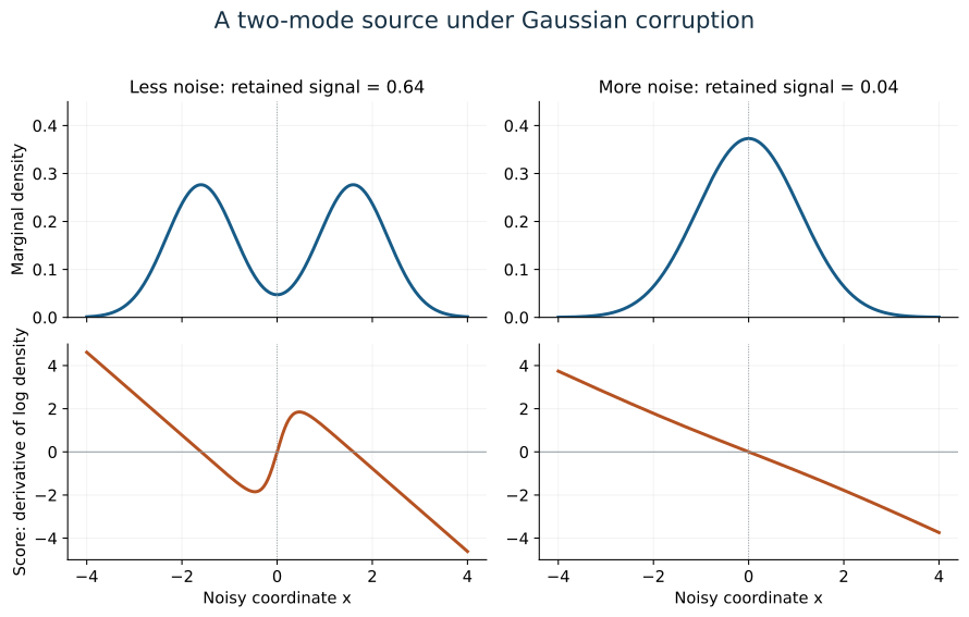
The figure plots the same analytic mixture at those two levels. Its lower panels show the score: the direction of increasing log probability.

5. Reverse stochastic evolution

For small steps the forward process has a continuous form

$$d{X}_t=f_t(X_t)dt+g_{t}d{W}_t,f_t(x)=-\frac{1}{2}b(t)x,g_t^2=b(t).$$

Here $b(t)$ is a rate, with discrete $b_k\simeq b(t)\Delta t$. The noise level $t$ is unrelated to training step. For spatially constant $g_t$, the density satisfies the Fokker–Planck equation ${\partial }_t{q}_t=-\nabla \cdot (f_t{q}_t)+(g_t^2/2)\Delta q_t$.

Under the smoothness, nonexplosion and positive-density hypotheses of diffusion time reversal, define increasing reverse time $u=T-t$ and $Y_u=X_{T-u}$. Its reverse drift is

$$d{Y}_u=\left[-f_{T-u}(Y_u)+g_{T-u}^2\nabla \log q_{T-u}(Y_u)\right]du+g_{T-u}d{\overline{W}}_u.$$

The noise is Brownian motion relative to the reverse-time information. The formula is a stated time-reversal theorem; checking its marginal equation is a useful verification, not a proof of the pathwise theorem.

Check. For stationary Ornstein–Uhlenbeck motion, $f(x)=-\gamma x$, $g^2=2\gamma$ and $q=\mathcal{N}(0,I)$, the score is $-x$. The reverse drift is $\gamma x-2\gamma x=-\gamma x$, identical to the forward drift. Merely reversing its sign would give the wrong process. For a nonstationary scalar Gaussian with mean $m_t$ and variance $v_t$, the reverse drift becomes $\gamma x-2\gamma (x-m_t)/v_t$.

An implemented generator replaces the score by an estimate, the terminal marginal by a prior, and continuous evolution by discrete steps. These give three separate errors: score fitting, prior mismatch and time discretization.

6. When thermodynamic quantities are defined

The formulas so far concern probabilities. A thermal interpretation also specifies an energy, bath temperature, mobility and their relation to noise. For example, $dX=-\gamma Xdt+\sqrt{2\gamma }dW$ can represent overdamped motion in a quadratic potential at unit temperature and appropriate mobility.

For this Ornstein–Uhlenbeck process, let $\pi =\mathcal{N}(0,I)$. Integration by parts, with sufficient decay at infinity, gives

$$\frac{d}{dt}D(q_t\Vert \pi )=-\gamma \int q_t{\Vert \nabla \log \frac{q_t}{\pi }\Vert }^{2}dx\le 0.$$

For a scalar Gaussian, the independent check is $D=\frac{1}{2}[m_t^2+v_t-1-\log v_t]$, with ${\dot{m}}_t=-\gamma m_t$, ${\dot{v}}_t=2\gamma (1-v_t)$. Therefore $\dot{D}=-\gamma [m_t^2+(v_t-1{)}^2/v_t]$. In the specified thermal realization, $k_{B}TD$ is excess nonequilibrium free energy. A decreasing probability discrepancy in a different model does not by itself measure heat.

A finite-state work identity

Specify energies $E_k(s)$ at inverse temperature ${\beta }_{\mathrm{th}}$, partition functions $Z_k$, and Gibbs laws ${\pi }_k(s)=e^{-{\beta }_{\mathrm{th}}{E}_k(s)}/Z_k$. Start in ${\pi }_0$. At each step switch $E_k$ to $E_{k+1}$ while holding $s_k$ fixed, with work $w_k=E_{k+1}(s_k)-E_k(s_k)$; then use a kernel preserving ${\pi }_{k+1}$.

The key identity is ${\pi }_k(s)e^{-{\beta }_{\mathrm{th}}{w}_k(s)}=(Z_{k+1}/Z_k){\pi }_{k+1}(s)$. Applying the preserving kernel and repeating makes the factors telescope:

$$\mathbb{E}{e}^{-{\beta }_{\mathrm{th}}W}=\frac{Z_K}{Z_0}=e^{-{\beta }_{\mathrm{th}}\Delta F},W=\sum _k{w}_k,\mathbb{E}W\ge \Delta F.$$

The last inequality is Jensen’s. The probability identity needs Gibbs preservation, which is weaker than detailed balance. Interpreting the protocol as a physical work experiment uses the specified energies and bath; it is not a consequence of fitting a denoising network.

Checkpoints with answers

1. Which distribution is Gaussian for arbitrary clean data? $q(x_k\mid x_0)$ at a fixed clean observation. Averaging over the unknown $q_0$ generally gives a non-Gaussian marginal $q_k$.

2. If ${\bar{\alpha }}_k=0.64$ and a predictor returns ${ϵ}_{\ast }=0.3$, what score does it imply? $s_k=-0.3/\sqrt{0.36}=-0.5$. The sign and scale are essential.

3. Does predicting the conditional mean produce a clean sample? Not generally. A mean between two modes can be atypical under the clean source. Sampling requires the specified reverse transitions.

4. What makes the work identity different from a generated path cost? It specifies energies, an equilibrium initial law, work during controlled switches and Gibbs-preserving transitions. A path’s negative log probability alone supplies none of these definitions.

What the week establishes

The conditional forward law and Gaussian posterior are exactly calculable. The variational bound has an explicit relative-entropy gap. At the population optimum, predicted noise determines the marginal score after the stated rescaling. The reverse equation then provides a generative route under its time-reversal hypotheses. Thermal interpretations apply to the separate specified physical constructions, with their additional assumptions.

The practical session — Laboratory 8

Varied: the time step, the terminal noise level and the training sample size — separately, never together, since the point is to attribute error to its source. Held fixed: the analytic model — Gaussian or two-Gaussian, for which the score is known in closed form — and the held-out set used for evaluation. Measured: moments and a stated distributional discrepancy on held-out samples, for a reverse sampler using the exact score and for one using a fitted predictor; and the relative-entropy decay against the closed-form Ornstein–Uhlenbeck expression, as a calibration.

Product: distributions, samples and errors with the three error sources separated and each attributed. Do not label the discrepancy of an arbitrary learned sampler as dissipated work: §6 states exactly what would have to be built first.

---

Connections to other parts of the wiki

• Week 1 supplies the relative entropy and its nonnegativity, which is what makes the variational bound a bound.
• Week 10 introduced a diffusion over parameters and a path cost distinct from entropy production; this week supplies the construction in which the thermal words are earned.
• Week 13 asked what a transition claim requires; this chapter asks the same question of a thermal claim, and answers it in §6.
• nn-llm-unit-4 — the block skeleton this note implements.

---

Start here · All weeks · Book and experiments · Previous week · Next week