TU · Collective physics · Five questions to investigate
Turbulence and anomalous dissipation
How does a nearly inviscid fluid keep converting motion into heat?
For a physicist entering another fieldSources checked 12 September 2026Editable working edition
The guiding question
Which properties of nonlinear transfer across scales survive as viscosity decreases, and which turbulent statistics require information beyond dimensional scaling?
Starting knowledge: Newton's second law, gradients, and energy conservation. No turbulence phenomenology is assumed initially.
Stirring a fluid creates motion on large scales. Nonlinear advection distorts that motion and creates finer spatial structure. Viscosity damps gradients most strongly, so transfer to fine scales can sustain conversion of macroscopic motion into heat even when viscosity is small.
The equations can be compact while their statistical consequences remain hard to derive. Predicting every eddy from an uncertain initial condition is one task; predicting averaged energy transfer and rare intense events is another. The mathematical global regularity problem for three-dimensional Navier–Stokes flow is also distinct: it asks whether appropriate smooth initial data always evolve smoothly. Solving a statistical model of turbulence would not automatically solve that theorem, and vice versa. [34]
What is known, and what is open
Energy balances and some scale-by-scale identities can be derived under explicit assumptions. Dimensional reasoning explains a celebrated inertial-range spectrum. It does not determine every exponent of velocity-difference statistics or the frequency of intense bursts. Intermittency names the uneven concentration of activity into unusually intense regions and times.
The small-viscosity limit can be singular: velocity gradients grow while the coefficient multiplying them shrinks. Onsager's theory relates persistent energy transfer to rough velocity fields. There are rigorous results on energy conservation and nonconservation for inviscid weak solutions, but existence of such solutions is not a complete derivation of the turbulent state selected by a physical forcing and vanishing viscosity. [35]
$\mathbf u$ is velocity, $p$ pressure enforcing incompressibility, $\rho_0$ mass density, $\nu$ kinematic viscosity, and $\mathbf f$ external force per unit mass. The advective term follows a fluid element through a nonuniform velocity field; it redistributes motion among scales.
For smooth periodic fields, multiplying by velocity and spatially averaging gives
The pressure and advection terms give no net volume energy change under these boundary conditions. In a statistically stationary forced state, average injection equals average dissipation $\varepsilon=\nu\langle|\nabla\mathbf u|^2\rangle$. The Reynolds number ${\rm Re}=UL/\nu$ compares advection with viscous smoothing at characteristic speed $U$ and length $L$.
If intermediate scales depend only on $\varepsilon$ and wave number $k$, dimensional analysis gives $E(k)=C\varepsilon^{2/3}k^{-5/3}$. The energy spectrum is normalized by $\langle|\mathbf u|^2\rangle/2=\int E(k)dk$; $C$ is dimensionless. The assumption of dependence on only those quantities is physics, not an algebraic identity.
Worked example: a shock keeps dissipating as viscosity vanishes
In one-dimensional Burgers flow, use
$$\partial_tu+u\partial_xu=\nu\partial_x^2u.$$
The stationary shock connecting $u(-\infty)=U$ to $u(+\infty)=-U$ is
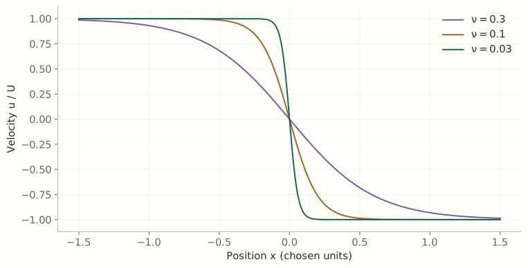
$$u(x)=-U\tanh\left(\frac{Ux}{2\nu}\right).$$
Its width shrinks as $\nu/U$ while its gradient grows as $U^2/\nu$. Direct integration gives
Thus the integrated dissipation remains finite as viscosity tends to zero. Energy flows in from the nonzero asymptotic velocities; this is not a freely decaying finite-energy configuration. Burgers flow supports compressive shocks, whereas incompressible three-dimensional turbulence has a different geometry and dynamics.
Exact stationary Burgers profiles with $U=1$ in chosen units. Smaller viscosity narrows the shock. Their equal integrated dissipation illustrates a singular limit, without modeling incompressible turbulence.
Insight. Setting $\nu=0$ before examining the gradients can remove the effect we wanted to understand. The correct question concerns the behavior of a sequence of viscous solutions and its energy balance.
Questions to investigate
Calibration questions have established answers. Diagnostics ask what follows inside a specified model or comparison. Extensions are bounded proposals whose novelty and feasibility need a focused literature check. Each answer should record its assumptions and limits.
TU-1 · Turbulence and anomalous dissipationCalibration
Can dissipation survive a coefficient tending to zero?
Do: Verify the shock solution and evaluate the dissipation integral analytically and numerically for several viscosities.
Check: Increase spatial resolution as the width decreases and include boundary energy flux. The integral tends to $2U^3/3$ without inventing a forcing term.
Meaning: A complete controlled example of a singular dissipation limit.
TU-2 · Turbulence and anomalous dissipationCalibration
What assumptions go into the minus-five-thirds spectrum?
Do: Derive the spectrum from units and its normalization. Then allow an outer length or a fluctuating local transfer rate as an extra input.
Check: Distinguish dimensional consistency from a uniqueness theorem. Define the scale interval in which forcing and viscosity are both negligible in the balance.
Meaning: Reveals exactly what the scaling argument explains and leaves undetermined.
TU-3 · Turbulence and anomalous dissipationDiagnostic
Can a measured structure function test the energy flux?
Do: In a homogeneous, isotropic, statistically stationary three-dimensional dataset, compare the longitudinal third-order velocity increment with the inertial-range prediction $\langle(\delta u_L)^3\rangle=-4\varepsilon r/5$. Here $\delta u_L=[\mathbf u(\mathbf x+\mathbf r)-\mathbf u(\mathbf x)]\cdot\hat{\mathbf r}$ is the velocity difference projected along the separation.
Check: Account for finite-viscosity, forcing, anisotropy, and finite-sampling corrections before declaring a violation.
Meaning: Tests a constrained flux relation rather than merely fitting a spectral slope. Its assumptions and limiting range are essential. [35]
TU-4 · Turbulence and anomalous dissipationDiagnostic
Which rare events dominate high moments?
Do: For a specified velocity dataset or synthetic model, compare $\langle|\delta u|^p\rangle$ for several orders $p$, including sensitivity to removing a small extreme tail.
Check: Use independent samples and convergence checks. A high-order moment with no stable estimate is not a measured exponent.
Meaning: Quantifies intermittency and distinguishes statistical uncertainty from failure of simple scaling.
TU-5 · Turbulence and anomalous dissipationExtension
Which coarse-graining scale reveals a stable energy flux?
Do: Filter one resolved velocity field at several lengths and derive the sub-filter transfer from the filtered equation. Compare it with the dissipation estimate.
Check: The filter definition and boundaries must be explicit; verify the resolved-plus-unresolved energy balance and vary the filter shape.
Meaning: A bounded robustness study of scale transfer. Existing coarse-graining theory is the starting benchmark, not a novelty claim.
Do TU-1 before a large fluid simulation. It gives an exact target for resolution and energy accounting. TU-2 then identifies the extra statistical information needed to move from a scaling law to an explanation of turbulent fluctuations.