Sem II Week 10 — The Zoo Beyond ℤ₂: Quantum Doubles, Modular Data, Chern–Simons

Sem II Week 8 solved the toric code: four anyons, four states on the torus, and $S$ and $T$ read off the string operators. This week leaves ${\mathbb{Z}}_2$ in two directions. Abelian Chern–Simons theory with an integer matrix $K$ contains the BF theory of Sem II Week 2, the toric code and the double semion of Sem II Week 7, and the chiral orders, the Laughlin state at $\nu =1/3$ among them, whose degeneracy, spins, charges and Hall response follow from one bracket. The quantum double of a finite group goes non-abelian: $S_3$ gives eight anyons, two of quantum dimension three. $S$ and $T$ are the invariants in which the two descriptions meet, and the edge of a chiral fluid is where the bulk data become a measurable current.

How to use this chapter

• In class: first hour, the bracket (2.3), the holonomy algebra (2.5) and the degeneracy (3.2)–(3.4); Problem 1. Second hour, flux attachment and braiding (4.1)–(4.2) with Figure 1, the spin (4.3), charge and Hall response (4.4)–(4.6), and §5 (Laughlin $\nu =1/3$, then the toric code matched to Week 8 and to Week 2 at $N=2$); Problems 2–3. Third hour, modular data (§6.1) with the properties of (6.3), the $D(S_3)$ count (§§7.2–7.3, Figure 2, Table 1) and the edge (§8, Figure 3); Problem 4. The seminar hour (§9) is Wen–Niu.
• For self-study: §§2.1, 4.4, 6.3, 7.4, 8.2, 10–12 and Problems 5⋆–8⋆. The one calculation to do alone: build the clock and shift matrices (3.2) for $K=\left(\begin{array}{cc}3& 2\\ 2& 3\end{array}\right)$ and verify (2.5) and irreducibility on the five states.
• Instructor checkpoint: two errors recur. With the weight (2.1) of conventions §10 and the orientation $dt\wedge dx\wedge dy$, the counterclockwise exchange of two quasiparticles $l$ gives $e^{-i\pi l^T{K}^{-1}l}$; the textbook $e^{+i\pi l^T{K}^{-1}l}$ belongs to the mirror convention, and copying it reverses the chirality of $\nu =1/3$, an error invisible for the toric code and for $D(G)$ (§4.4). And a charge bound to a flux $g$ of $D(G)$ carries an irreducible representation of the centralizer $Z(g)$ only: counting irreducible representations of $S_3$ for each of its three classes gives nine anyons, and the correct count is eight (§7.2).

0. Reading

Primary: Wen, Zee, “A classification of Abelian quantum Hall states and matrix formulation of topological fluids”, Phys. Rev. B 46 (1992) 2290: $K$ and $t$ as the data of an abelian Hall fluid. Kitaev, quant-ph/9707021, cited in the arXiv numbering (§§5 and 7 in the Annals version): §4, the lattice model on the group algebra of a finite group $G$, and §6, “Topological operators, braiding, and fusion”, for the flux–charge anyons of §7. Kitaev, Ann. Phys. 321 (2006) 2 [cond-mat/0506438], App. E, as a reference for $S$, $T$, the Verlinde formula and the relation of $c$ to the spins.

Secondary: Wen, Quantum Field Theory of Many-Body Systems (2004), the chapters on the fractional quantum Hall effect and its edge; Preskill, Lecture Notes, ch. 9, as a companion to §6; Laughlin, Phys. Rev. Lett. 50 (1983) 1395 (the $\nu =1/m$ wave function and its fractional charge); Witten, “The Chern–Simons function and the quantum Hall effect”, to appear in Bull. Amer. Math. Soc. [arXiv:2609.21182], §§3–4: the Hall level quantized from the effective action alone, odd levels needing a spin structure, inflow at the edge, and the emergent-field model $\frac{k}{4\pi }AdA+\frac{s}{2\pi }Ada+\frac{r}{4\pi }ada$, which is (2.1) with $K=r$, $t=s$ and a background level $k$, so that ${\sigma }_{xy}=(k-s^2/r)e^2/2\pi$ by (4.6); his $\nu =1/3$ example, $(k,s,r)=(0,1,-3)$, is the mirror image of the $K=3$ of §5. See 2026-witten-chern-simons-quantum-hall.

Seminar paper: Wen, Niu, “Ground-state degeneracy of the fractional quantum Hall states in the presence of a random potential and on high-genus Riemann surfaces”, Phys. Rev. B 41 (1990) 9377 (§9).

Optional research reading: Wen, Phys. Rev. B 41 (1990) 12838 (the chiral Luttinger-liquid edge of §8); Arovas, Schrieffer, Wilczek, Phys. Rev. Lett. 53 (1984) 722 (the fractional statistics of quasiholes); Witten, Commun. Math. Phys. 121 (1989) 351 (Chern–Simons theory as a topological field theory); Coste, Gannon, Ruelle, Nucl. Phys. B 581 (2000) 679 [hep-th/0001158] (modular data of finite-group doubles, §7.4); Dijkgraaf, Witten, Commun. Math. Phys. 129 (1990) 393.

Proof-status labels follow note-quality-template §4. The $K$-matrix weight (2.1) is the Chern–Simons weight of conventions §10, the anyon data follow Week 7 (6.4)–(6.8), and the conventions (4.3), (6.1) and (7.4) for spins, $S$ and $T$ are those recorded in conventions §§9–10.

1. Motivation and setting

Week 7 found a second ${\mathbb{Z}}_2$ order with the degeneracy of the toric code and different spins, so a topological-order needs more data than its degeneracy. The physical question of the week is which data suffice. For the abelian Chern–Simons theories and for the deconfined phases $D(G)$ of lattice gauge theory with a finite gauge group, the answer is a short list: the anyon types with their fusion, the spins and the braiding, organized into $T$ and $S$. We derive the list from the action for the first family and from the gauge structure for the second, and check that the two agree at ${\mathbb{Z}}_N$.

2. Abelian Chern–Simons theory with a $K$-matrix

2.1 The action and the integrality of $K$ [Proved, given the extension to a 4-manifold.]

Let $M$ be a closed oriented 3-manifold, $a^I$ ($I=1,\dots ,n$) $U(1)$ gauge fields with fluxes in $2\pi \mathbb{Z}$, and $K$ a real symmetric $n\times n$ matrix with $\det K\ne 0$. The weight is

$$Z(M)=\int \prod _I\mathcal{D}{a}^I\exp (\frac{i}{4\pi }{K}_{IJ}{\int }_M{a}^I\wedge d{a}^J).\text{\hspace{1em}(2.1)}$$

For $n=1$ this is the Chern–Simons weight of conventions §10 at level $k=K$. For $K=\left(\begin{array}{cc}0& N\\ N& 0\end{array}\right)$ and $(a^1,a^2)=(a,b)$ it is $\frac{iN}{4\pi }\int (a\wedge db+b\wedge da)=\frac{iN}{2\pi }\int b\wedge da$, the BF weight of Week 2 (2.1), by the identity $\int a\wedge db=\int b\wedge da$ of Week 2 §2.1.

When fluxes are present $a\wedge da$ is not built from global forms (F1), and the clean definition extends the fields to an oriented 4-manifold $X$ with $\partial X=M$, which exists for every $M$ and every choice of bundles [Stated], and sets $\frac{1}{4\pi }{K}_{IJ}{\int }_M{a}^I\wedge d{a}^J\equiv \frac{1}{4\pi }{K}_{IJ}{\int }_X{F}^I\wedge F^J$. Two extensions differ by a closed 4-manifold $Y$, and with $c^I=F^I/2\pi$ the weight changes by

$$\exp (i\pi K_{IJ}{\int }_Y{c}^I\wedge c^J)=\exp \left(i\pi \right[\sum _I{K}_{II}{\int }_Y{c}^I\wedge c^I+2\sum _{I<J}{K}_{IJ}{\int }_Y{c}^I\wedge c^J\left]\right).$$

The integrals are integers, and ${\int }_{Y}c\wedge c$ is even on spin manifolds and odd on some others (conventions §10: $Q=\frac{1}{2}\int c_1\wedge c_1$ is an integer on spin manifolds and in $\frac{1}{2}\mathbb{Z}$ in general). Therefore the weight is independent of $X$ for every $M$ if and only if $K_{IJ}\in \mathbb{Z}$ and every diagonal entry $K_{II}$ is even. With an odd diagonal entry it is well defined only on spin manifolds, and the theory depends on a spin structure. BF theory has zero diagonal and any integer $N$, as Week 2 found. §4.2 shows what an odd entry means physically: a local fermion.

2.2 The Hamiltonian form and the bracket [Computed.]

On $\mathbb{R}\times \Sigma$ with orientation $dt\wedge dx\wedge dy$ and ${ϵ}^{xy}={ϵ}_{xy}=+1$, the Minkowski weight is $e^{iS}$ with $S=\frac{1}{4\pi }{K}_{IJ}\int d^{3}x{ϵ}^{\mu \nu \rho }{a}_{\mu }^I{\partial }_{\nu }{a}_{\rho }^J$ (a topological term has the same expression in both signatures, conventions §10). Separating the terms with one time index and integrating by parts, as Week 2 (3.1) did for BF,

$$S=\frac{1}{4\pi }\int dt{d}^{2}x[-K_{IJ}{ϵ}^{ij}{a}_i^I{\dot{a}}_j^J+2a_t^I{K}_{IJ}{f}^J],f^J\equiv {ϵ}^{ij}{\partial }_i{a}_j^J;\text{\hspace{1em}(2.2)}$$

we checked with sympy that (2.1) and (2.2) give identical Euler–Lagrange equations for a general symmetric $2\times 2$ $K$. The $a_t^I$ impose $f^J=0$, since $K$ is invertible. The kinetic term is $\frac{1}{4\pi }{K}_{IJ}(a_y^I{\dot{a}}_x^J-a_x^I{\dot{a}}_y^J)=\frac{1}{2\pi }{K}_{IJ}{a}_y^I{\dot{a}}_x^J$ plus a total time derivative, so the momentum of $a_x^J$ is $\frac{1}{2\pi }{K}_{JI}{a}_y^I$, and $[a_x^J,\frac{1}{2\pi }{K}_{J^{\prime }I}{a}_y^I]=i{\delta }_{J^{\prime }}^J{\delta }^2$ gives

$$[a_i^I(\mathbf{x}),a_j^J(\mathbf{y})]=2\pi i(K^{-1}{)}^{IJ}{ϵ}_{ij}{\delta }^2(\mathbf{x}-\mathbf{y}).\text{\hspace{1em}(2.3)}$$

For BF, $(K^{-1}{)}^{12}=1/N$ and (2.3) is Week 2 (3.3); at level $k$, $[a_x,a_y]=\frac{2\pi i}{k}{\delta }^2$. A quasiparticle of charge vector $l\in {\mathbb{Z}}^n$ at rest at ${\mathbf{x}}_0$ is the Wilson line $\exp (i{l}_I\int a^I)$ along its worldline, which adds $l_I{a}_t^I{\delta }^2(\mathbf{x}-{\mathbf{x}}_0)$ to the Lagrangian density, and the equation of $a_t^I$ becomes

$$\frac{1}{2\pi }{K}_{IJ}{f}^J+l_I{\delta }^2(\mathbf{x}-{\mathbf{x}}_0)=0,\text{that is,}f=-2\pi K^{-1}l{\delta }^2(\mathbf{x}-{\mathbf{x}}_0).\text{\hspace{1em}(2.4)}$$

2.3 Holonomies and the charge lattice [Computed.]

For closed curves γ, γ′ on Σ let $W_l(\gamma )=\exp (i{l}_I{\oint }_{\gamma }{a}^I)$. By (2.3), $[l\cdot {\oint }_{\gamma }a,l^{\prime }\cdot {\oint }_{{\gamma }^{\prime }}a]=2\pi i{l}^T{K}^{-1}{l}^{\prime }\gamma \cdot {\gamma }^{\prime }$ with the intersection number of Week 2 (3.5), and $e^X{e}^Y=e^Y{e}^X{e}^{[X,Y]}$ gives

$$W_l(\gamma )W_{l^{\prime }}({\gamma }^{\prime })=e^{-2\pi i{l}^T{K}^{-1}{l}^{\prime }\gamma \cdot {\gamma }^{\prime }}{W}_{l^{\prime }}({\gamma }^{\prime })W_l(\gamma ),\text{\hspace{1em}(2.5)}$$

which for $l=(1,0)$, $l^{\prime }=(0,1)$ and BF is $WV={\omega }^{-\gamma \cdot {\gamma }^{\prime }}VW$, Week 2 (3.6). For $l=Kv$ with $v\in {\mathbb{Z}}^n$, (2.3) gives $W_{Kv}(\gamma )a^J{W}_{Kv}(\gamma {)}^{-1}=a^J-2\pi v^J{\delta }_{\gamma }$, a large gauge transformation, as in Week 2 (3.8); so $W_{Kv}(\gamma )$ acts trivially on physical states (for odd $K_{II}$ up to a sign, F2). Line labels therefore live in the discriminant group

$$\mathcal{A}={\mathbb{Z}}^n/K{\mathbb{Z}}^n,|\mathcal{A}|=|\det K|.\text{\hspace{1em}(2.6)}$$

The order follows from the Smith normal form $K=UDV$ with $U,V\in GL(n,\mathbb{Z})$ and $D=\mathrm{diag}(d_1,\dots ,d_n)$: ${\mathbb{Z}}^n/K{\mathbb{Z}}^n\cong {\oplus }_i{\mathbb{Z}}_{|d_i|}$, of order $\prod |d_i|=|\det K|$ [Proved]. We checked $|\mathcal{A}|=|\det K|$ and the invariant factors for every $K$ of this note.

3. Ground-state degeneracy $|\det K{|}^g$ [Proved.]

On $T^2$ with the cycles of Week 2 Figure 1, $C_x\cdot C_y=+1$, the solutions of $f=0$ modulo small gauge transformations are $a^I={\theta }^{I}dx/L_x+{\varphi }^{I}dy/L_y$, with periods ${\theta }^I={\oint }_{C_x}{a}^I$ and ${\varphi }^I={\oint }_{C_y}{a}^I$ defined modulo $2\pi$. The kinetic term of (2.2) reduces to

$$L=\frac{1}{2\pi }{\varphi }^{T}K\dot{\theta },\text{\hspace{1em}(3.1)}$$

$n$ copies of Week 2 (3.9) coupled by $K$. The momentum of θ is $p=K\varphi /2\pi$; the periodicity of θ quantizes $p\in {\mathbb{Z}}^n$, so $\varphi =2\pi K^{-1}p$, and the periodicity $\varphi \to \varphi +2\pi v$ identifies $p\sim p+Kv$. The physical states are $|\lambda ⟩$, $\lambda \in \mathcal{A}$, and since $e^{il\cdot \theta }$ raises $p$ by $l$ while $e^{il\cdot \varphi }=e^{2\pi i{l}^T{K}^{-1}p}$,

$$U_l|\lambda ⟩\equiv W_l(C_x)|\lambda ⟩=|\lambda +l⟩,V_l|\lambda ⟩\equiv W_l(C_y)|\lambda ⟩=e^{2\pi i{l}^T{K}^{-1}\lambda }|\lambda ⟩.\text{\hspace{1em}(3.2)}$$

These satisfy (2.5) with $C_x\cdot C_y=1$ and are well defined on $\mathcal{A}$, since $e^{2\pi i{l}^T{K}^{-1}Kv}=1$. They act irreducibly: the phases $\lambda \mapsto e^{2\pi i{l}^T{K}^{-1}\lambda }$ separate the points of $\mathcal{A}$ by the nondegeneracy lemma of §6.2, so an operator commuting with every $V_l$ is diagonal, and the $U_l$ act transitively, so a diagonal operator commuting with them is a multiple of 1. Therefore

$$\mathrm{GSD}(T^2)=|\det K|.\text{\hspace{1em}(3.3)}$$

On ${\Sigma }_g$ the symplectic basis $A_i,B_i$ of Week 2 Figure 2 gives one copy of (3.1) per handle, and

$$\boxed{\mathrm{GSD}({\Sigma }_g)=|\det K{|}^g}\text{\hspace{1em}(3.4)}$$

For BF, $|\det K|=N^2$ and (3.4) is Week 2 (4.2); for $K=q$ it is the $q^g$ of Wen and Niu (§9). We built (3.2) as explicit matrices for the $K$ of §5 and of Problems 1, 2 and 5⋆, and checked (2.5) and a one-dimensional commutant on $T^2$, and on ${\Sigma }_2$ with $|\det K{|}^2$ states.

4. Braiding, spin and charge from the Gauss law

4.1 Flux attachment and mutual statistics [Computed.]

By (2.4) a quasiparticle $l$ carries the fluxes $\oint a=-2\pi K^{-1}l$ around any counterclockwise loop that encloses it (Figure 1). A second quasiparticle $l^{\prime }$ carried once counterclockwise around it is the operator $W_{l^{\prime }}(C)$ on that loop, and it acquires the Aharonov–Bohm phase

$$B(l^{\prime },l)=\exp (i{l}^{\prime T}(-2\pi K^{-1}l))=\exp (-2\pi i{l}^{\prime T}{K}^{-1}l).\text{\hspace{1em}(4.1)}$$

In spacetime, the Gaussian integral of Week 2 §5.1 with the sources $l{\delta }_C+l^{\prime }{\delta }_{C^{\prime }}$ has the stationary point $da=-2\pi K^{-1}(l{\delta }_C+l^{\prime }{\delta }_{C^{\prime }})$, and the cross term of its on-shell exponent gives

$$⟨W_l(C)W_{l^{\prime }}(C^{\prime })⟩=\exp (-2\pi i{l}^T{K}^{-1}{l}^{\prime }\mathrm{Lk}(C,C^{\prime }))\times (\text{self-linking factors}).\text{\hspace{1em}(4.2)}$$

For BF with $l=(e,0)$, $l^{\prime }=(0,m)$ this is ${\omega }^{-em\mathrm{Lk}}$, Week 2 (5.4). A counterclockwise circuit in the $xy$-plane around a static worldline has $\mathrm{Lk}=+1$ (Week 2 Figure 3; a numerical Gauss integral confirms it with the frame $(x,y,t)$, which is positive because $dx\wedge dy\wedge dt=dt\wedge dx\wedge dy$), so (4.1) and (4.2) agree. $B$ is symmetric and bimultiplicative, depends on $l,l^{\prime }$ only through their classes in $\mathcal{A}$, and $B(Kv,l^{\prime })=e^{-2\pi iv\cdot l^{\prime }}=1$: the particles $Kv$ braid trivially with everything, and they are the local excitations. The mutual-statistics angle is $2\pi l^T{K}^{-1}{l}^{\prime }$, which is $2\pi (K^{-1}{)}_{ab}$ for $l=e_a$, $l^{\prime }=e_b$.

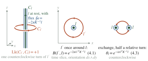
Figure 1. Flux attachment. A static quasiparticle drags the flux tube (2.4); a counterclockwise circuit of $l^{\prime }$ links its worldline with $\mathrm{Lk}=+1$ and picks up the phase (4.1); half a relative turn of two identical quasiparticles gives the spin (4.3).

4.2 Topological spin and the local fermion [Computed in the adiabatic limit.]

For slow motion in the plane the phase (4.1) accumulates continuously with the relative angle φ of the two particles: integrating out $a$ leaves each pair with the effective coupling $-l^T{K}^{-1}{l}^{\prime }\dot{\phi }$, which reproduces (4.1) for $\Delta \phi =2\pi$. (It is half the sum of the two Aharonov–Bohm couplings, $l^{\prime }$ in the flux of $l$ and $l$ in that of $l^{\prime }$: the $\frac{1}{2}$ of the on-shell exponent of §4.1.) Two identical particles exchanged counterclockwise make half a relative turn, $\Delta \phi =\pi$, so the exchange phase, which is the spin ${\theta }_X=R(X,X)$ of Week 7 (6.8), is

$$\boxed{{\theta }_l=\exp (-i\pi l^T{K}^{-1}l),B(l,l^{\prime })=\frac{{\theta }_{l+l^{\prime }}}{{\theta }_l{\theta }_{l^{\prime }}}=\exp (-2\pi i{l}^T{K}^{-1}{l}^{\prime })}\text{\hspace{1em}(4.3)}$$

The second equality is the monodromy relation of Week 7 §6.4, now an identity of quadratic forms; we checked it for every pair of labels and every $K$ of this note. The statistics angle is $\pi l^T{K}^{-1}l$, which is $\pi (K^{-1}{)}_{aa}$ for $l=e_a$; in our orientation it is measured clockwise (§4.4).

Shifting a label by a local particle gives ${\theta }_{l+Kv}={\theta }_l\exp (-i\pi (2v\cdot l+v^{T}Kv))={\theta }_l(-1{)}^{v^{T}Kv}$, and $v^{T}Kv\equiv {\sum }_I{K}_{II}{v}_I$ mod 2. So θ is a function on $\mathcal{A}$ if and only if every $K_{II}$ is even, the bosonic condition of §2.1. If $K_{II}$ is odd, the local particle $K{e}_I$ has $\theta =-1$: the theory contains a local fermion, and spins are defined only up to its sign.

4.3 Electric charge and Hall response [Computed.]

Couple the theory to a background $A$ through $\frac{1}{2\pi }{t}_I\int A\wedge d{a}^I$, with an integer charge vector $t$. The charge density is $\delta S/\delta A_t=\frac{1}{2\pi }{t}^{T}f$, and by (2.4) the charge of $l$ is

$$Q_l=\frac{1}{2\pi }{t}^T\int f=-t^T{K}^{-1}l.\text{\hspace{1em}(4.4)}$$

Local particles have $Q_{Kv}=-t\cdot v\in \mathbb{Z}$. The $a$ equation $\frac{1}{2\pi }(Kda+tdA)=0$ gives $a=-K^{-1}tA$, and substituting,

$$S_{\mathrm{resp}}=\frac{1}{4\pi }\nu \int A\wedge dA-\frac{1}{2\pi }\nu \int A\wedge dA=-\frac{\nu }{4\pi }\int A\wedge dA,\nu \equiv t^T{K}^{-1}t.\text{\hspace{1em}(4.5)}$$

This is a Chern–Simons term of level $-\nu$ for the background, and Sem I Week 12 §8.2 converts a level into a Hall conductivity, so

$${\sigma }_{xy}=-\nu \frac{e^2}{2\pi },\rho =-\frac{\nu }{2\pi }{B}_z,\text{\hspace{1em}(4.6)}$$

the second relation being the Středa formula of that section.

4.4 The orientation, once [Proved, given §§4.1–4.3.]

For positive-definite $K$, the weight (2.1) and the orientation $dt\wedge dx\wedge dy$ give three linked statements: the counterclockwise exchange phase is $e^{-i\pi l^T{K}^{-1}l}$; by (4.4)–(4.6) with $K=3$, $t=1$, the local particle $l=3$ has charge $-1$ and density $\nu B_z/2\pi$ in a field $B_z>0$, so the theory describes electrons in a field along $+\hat{z}$, with ${\sigma }_{xy}<0$ as for any negative carriers; and the edge modes run clockwise (§8.2). Much of the quantum Hall literature writes the Lagrangian with $-\frac{1}{4\pi }Kada$, the mirror image $K\to -K$, in which the counterclockwise exchange gives $e^{+i\pi l^T{K}^{-1}l}$, ${\sigma }_{xy}=+\nu e^2/2\pi$ and the edges run counterclockwise. The orientation-independent content is the pairing of the two senses: the exchange measured in the sense in which the edge modes of a definite $K$ propagate gives $e^{+i\pi l^T|K{|}^{-1}l}$. The toric code and the untwisted $D(G)$ are their own mirror images up to relabelling (for $D(S_3)$, $G\leftrightarrow H$), and for them the convention never shows.

Physical picture. A quasiparticle of the $K$-matrix fluid is a charge of the emergent gauge fields bound to a flux tube of them, (2.4), and every number of §4 is an Aharonov–Bohm phase of that composite: braiding is a charge encircling a flux, the spin is half of it, and the electric charge (4.4) is the flux read through $t$. This is exact in (2.1). A Hall bar shows the response (4.6), a plateau at $|{\sigma }_{xy}|=\nu e^2/h$, and through (4.4) quasiparticles of fractional charge; the braiding phases need interferometry, and §4.4 decides only which way round the interferometer a phase is quoted.

5. Two worked examples [Computed.]

5.1 Laughlin $\nu =1/3$: $K=3$, $t=1$

Here $\mathcal{A}={\mathbb{Z}}_3$ and $\mathrm{GSD}({\Sigma }_g)=3^g$. With $K^{-1}=\frac{1}{3}$, (4.3) and (4.4) give, for the representatives $l=0,1,2$ and the shifted ones,

$l$	$Q_l$	$l^T{K}^{-1}l$	${\theta }_l$
0	0	0	1
$\pm 1$	$\mp \frac{1}{3}$	$\frac{1}{3}$	$e^{-i\pi /3}$
2	$-\frac{2}{3}$	$\frac{4}{3}$	$e^{-4\pi i/3}=-e^{-i\pi /3}$
3	$-1$	3	$-1$

The labels 2 and $-1$ are one class of $\mathcal{A}$ and their spins differ by the sign of the electron $l=3$, as §4.2 requires for odd $K$; the electron has charge $-1$, spin $-1$, and braids trivially, $B(3,l)=e^{-2\pi il}=1$. The braiding phases are well defined on $\mathcal{A}$: $B(1,1)=e^{-2\pi i/3}$ and $B(1,-1)=e^{+2\pi i/3}$. The quasihole $l=-1$ has charge $+\frac{1}{3}$ and statistics angle $\frac{\pi }{3}$ (two quasiholes exchanged clockwise acquire $e^{i\pi /3}$), and ${\sigma }_{xy}=-\frac{1}{3}{e}^2/2\pi$: the threefold degeneracy, the charge $e/3$ and the angle $\pi /3$ come from the single number $K=3$ (every entry computed in exact rational arithmetic).

5.2 The toric code: $K=\left(\begin{array}{cc}0& 2\\ 2& 0\end{array}\right)$

This is Week 2 at $N=2$ in the basis $(a^1,a^2)=(a,b)$. Then $\det K=-4$, the Smith form is $\mathrm{diag}(2,2)$, $\mathcal{A}={\mathbb{Z}}_2\times {\mathbb{Z}}_2$, $\mathrm{GSD}({\Sigma }_g)=4^g$ as in Week 2 (4.2) and Week 8, and $K^{-1}=\frac{1}{2}\left(\begin{array}{cc}0& 1\\ 1& 0\end{array}\right)$, so $l^T{K}^{-1}{l}^{\prime }=\frac{1}{2}(l_1{l}_2^{\prime }+l_2{l}_1^{\prime })$. The labels follow Week 2 §5.2: the line $W=e^{i\oint a}$ ends on violations of the Gauss law $f_b=0$, the star term, so $e=(1,0)$; the line $U=V^{†}=e^{-i\oint b}$ of Week 2 (5.5) ends on violations of $f_a=0$, the plaquette term, so $m=(0,-1)\equiv (0,1)$; and $\epsilon =e+m=(1,-1)\equiv (1,1)$. By (4.3),

$${\theta }_l=e^{-i\pi l_1{l}_2}:{\theta }_1={\theta }_e={\theta }_m=1,{\theta }_{\epsilon }=-1;B(e,m)=B(e,\epsilon )=B(m,\epsilon )=-1,B(e,e)=B(m,m)=B(\epsilon ,\epsilon )=1.$$

These are the anyons $e,m,\epsilon$ of Week 8 §4, with the braiding of its §4.3 and the spins of its §4.4, and of conventions §9: a boson pair with mutual braiding $-1$ and their fermionic composite, and the spins of Week 7 Table 2 at $k=0$. For general $N$ the label $l=(a,-b)$ is $e^a{m}^b$, with $e$ at the end of the string $W$, where Week 8 F4 places physical charge $+1$; then $l^T{K}^{-1}l=-2ab/N$, ${\theta }_{e^a{m}^b}={\omega }^{ab}$ and $B(e,m)=\omega$ as in conventions §9, both checked at $N=3$.

5.3 The double semion: $K=\mathrm{diag}(2,-2)$

Again $\mathcal{A}={\mathbb{Z}}_2\times {\mathbb{Z}}_2$ and $\mathrm{GSD}=4^g$, and ${\theta }_{(l_1,l_2)}=e^{-i\pi (l_1^2-l_2^2)/2}$. With $s=(0,1)$, $\bar{s}=(1,0)$ and $b=(1,1)$: ${\theta }_s=i$, ${\theta }_{\bar{s}}=-i$, ${\theta }_b=1$, $s+\bar{s}=b$, $2s=(0,2)\equiv 0$, $B(s,s)=-1$, $B(s,\bar{s})=1$ and $B(b,s)=-1$. This is Week 7 Table 2 at $k=1$; in our orientation the level $+2$ factor carries $\bar{s}$.

6. Modular data

6.1 Definitions and relations [Stated — refs: Kitaev App. E; checked in every example.]

For a theory with anyon labels $a$ (0 the vacuum), fusion coefficients $N_{ab}^c$, duals $\bar{a}$, quantum dimensions $d_a$ ($d_a=1$ for abelian anyons) and spins ${\theta }_a$, we define

$$T_{ab}={\theta }_a{\delta }_{ab},S_{ab}=\frac{1}{\mathcal{D}}\sum _c{N}_{a\bar{b}}^c{d}_c\frac{{\theta }_c}{{\theta }_a{\theta }_b},{\mathcal{D}}^2=\sum _a{d}_a^2.\text{\hspace{1em}(6.1)}$$

For abelian anyons $S_{ab}={\mathcal{D}}^{-1}B(a,\bar{b})={\mathcal{D}}^{-1}B(a,b{)}^{\ast }$. In a modular theory these matrices obey

$$S=S^T,S{S}^{†}=1,S^2=C,(ST{)}^3=\Theta S^2,\Theta =\frac{1}{\mathcal{D}}\sum _a{d}_a^2{\theta }_a=e^{2\pi ic/8},d_a=\frac{S_{0a}}{S_{00}},N_{ab}^c=\sum _x\frac{S_{ax}{S}_{bx}{S}_{cx}^{\ast }}{S_{0x}},\text{\hspace{1em}(6.2)}$$

with $C_{ab}={\delta }_{\bar{a}b}$ and $c$ the chiral central charge of the edge. On $T^2$, $S$ and $T$ represent the rotation $(x,y)\to (y,-x)$ and the Dehn twist on the ground space, $T$ up to the phase $e^{-2\pi ic/24}$ that (6.1) drops [Stated]. Week 8 §5 obtains the toric-code pair this way, and its §5.2 quotes (6.1) as Kitaev’s definition. The pair $(S,T)$ is the fingerprint of the order: it fixes the fusion rules through the Verlinde formula and $c$ mod 8 through Θ.

6.2 The $K$-matrix theory [Proved for unitarity and $S^2=C$; (ST)³ and (6.4) Stated — refs: Milgram; checked numerically.]

By (4.3) and (6.1),

$$S_{l{l}^{\prime }}=\frac{1}{\sqrt{|\det K|}}{e}^{2\pi i{l}^T{K}^{-1}{l}^{\prime }},T_{ll}=e^{-i\pi l^T{K}^{-1}l}.\text{\hspace{1em}(6.3)}$$

Nondegeneracy lemma. If $l^T{K}^{-1}{l}^{\prime }\in \mathbb{Z}$ for every $l^{\prime }\in {\mathbb{Z}}^n$, then $K^{-1}l\in {\mathbb{Z}}^n$, so $l\in K{\mathbb{Z}}^n$ and $l=0$ in $\mathcal{A}$. The rows of $S$ are therefore $|\mathcal{A}|$ distinct characters of $\mathcal{A}$, and character orthogonality gives $(S{S}^{†}{)}_{l{l}^{\prime \prime }}=|\mathcal{A}{|}^{-1}{\sum }_{l^{\prime }}{e}^{2\pi i(l-l^{\prime \prime }{)}^T{K}^{-1}{l}^{\prime }}={\delta }_{l{l}^{\prime \prime }}$ and $(S^2{)}_{l{l}^{\prime \prime }}={\delta }_{l,-l^{\prime \prime }}$, which is $C$. For even $K$ we verified $(ST{)}^3=\Theta S^2$ numerically for $K=2$, $\left(\begin{array}{cc}2& 1\\ 1& 2\end{array}\right)$ and the four matrices of §5.2, §5.3 and Problems 2 and 6⋆, and in each case

$$\Theta =\frac{1}{\sqrt{|\det K|}}\sum _{l\in \mathcal{A}}{e}^{-i\pi l^T{K}^{-1}l}=e^{-2\pi i\sigma (K)/8},\text{\hspace{1em}(6.4)}$$

with σ the signature; the general identity is Milgram’s formula for even lattices [Stated]. In the counterclockwise convention, then, $c\equiv -\sigma (K)$ mod 8, and §8.2 confirms it independently: $\sigma (K)$ net modes run clockwise. For odd $K$, $S$ is still well defined and unitary on $\mathcal{A}$, but $T$ is defined only up to the local-fermion sign, and the relations involving $T$ need a spin structure (F2).

6.3 The examples [Computed; the relations (6.2) checked numerically.]

For the toric code, (6.3) with the labels of §5.2 reproduces Week 8 (5.5) and (5.7), $(S_{\mathrm{TC}}{)}_{ab}=\frac{1}{2}B(a,b)$ and $T_{\mathrm{TC}}=\mathrm{diag}(1,1,1,-1)$ in the order $(1,e,m,\epsilon )$, and the group formula (7.5) at $G={\mathbb{Z}}_2$ returns the same $S_{\mathrm{TC}}$ (checked): the $K$-matrix and quantum-double descriptions agree. For the double semion, in the order $(1,b,s,\bar{s})$,

$$S_{\mathrm{DS}}=\frac{1}{2}\left(\begin{array}{cccc}1& 1& 1& 1\\ 1& 1& -1& -1\\ 1& -1& -1& 1\\ 1& -1& 1& -1\end{array}\right),T_{\mathrm{DS}}=\mathrm{diag}(1,1,i,-i),$$

and both theories have $\Theta =1$, so both are non-chiral. They share fusion rules and degeneracy and differ in $T$, and also in $S$: $(S_{\mathrm{DS}}{)}_{ss}=-\frac{1}{2}$, the self-braiding $B(s,s)=-1$, while every diagonal entry of $S_{\mathrm{TC}}$ is $+\frac{1}{2}$, so no relabelling maps one pair onto the other. For $\nu =1/3$, (6.3) gives $S=\frac{1}{\sqrt{3}}\left(\begin{array}{ccc}1& 1& 1\\ 1& \omega & \bar{\omega }\\ 1& \bar{\omega }& \omega \end{array}\right)$ with $\omega =e^{2\pi i/3}$, unitary, with $S^2=C$ exchanging the labels 1 and 2.

7. The quantum double $D(G)$ and the anyons of $S_3$

7.1 The lattice model in outline [Stated — refs: Kitaev, quant-ph/9707021, §4 in the arXiv numbering.]

Place a $G$-valued variable on each oriented link, with Hilbert space $\mathbb{C}[G]$ per link. At each vertex, $A_v=|G{|}^{-1}{\sum }_h{A}_v^h$ averages over the gauge transformations $A_v^h$ by $h\in G$ at $v$; on each plaquette, $B_p$ projects onto configurations whose ordered product around $p$ is the identity; $H=-{\sum }_v{A}_v-{\sum }_p{B}_p$. For $G={\mathbb{Z}}_2$, $A_v=\frac{1}{2}(1+\prod X)$ and $B_p=\frac{1}{2}(1+\prod Z)$, and $H$ is half the toric code of conventions §9 plus a constant. The ground states are the gauge-invariant superpositions of flat configurations, one per gauge orbit of holonomies, so $\mathrm{GSD}(\Sigma )=|\mathrm{Hom}({\pi }_1(\Sigma ),G)/G|$. This is the untwisted Dijkgraaf–Witten theory of Week 7 §6.1 in Hamiltonian form: $Z(\Sigma \times S^1)=|\mathrm{Hom}({\pi }_1(\Sigma )\times \mathbb{Z},G)|/|G|={\sum }_{\varphi }|\mathrm{Stab}(\varphi )|/|G|$, the sum running over homomorphisms φ of ${\pi }_1(\Sigma )$ and $\mathrm{Stab}(\varphi )$ being the elements that commute with its image, and by the orbit–stabilizer theorem this is the number of orbits [Proved].

7.2 Anyons as fluxes with centralizer charges [Proved for the labels, the count and $\mathcal{D}$.]

A plaquette with $B_p$ violated carries a flux, the holonomy $g\ne e$ around $p$ read from a base vertex $v_0$ (Figure 2). A gauge transformation $h$ at $v_0$ maps $g\to hg{h}^{-1}$, so the gauge-invariant label of a flux is its conjugacy class $C$. A charge at $v_0$ transforms under the gauge transformations there; in the presence of the flux $g$, those that leave $g$ fixed form the centralizer $Z(g)=\{h:hg{h}^{-1}=g\}$, and the others move $g$ around its class. The composite is labelled by $C$ and an irreducible representation α of $Z(g_C)$ (centralizers of conjugate elements are conjugate, so any representative will do), and its internal space, spanned by $|g^{\prime },v⟩$ with $g^{\prime }\in C$ and $v$ in the space of α, has dimension $|C|\dim \alpha$:

$$\text{anyons}⟷(C,\alpha ),\alpha \in \mathrm{Irr}Z(g_C),d_{(C,\alpha )}=|C|\dim \alpha .\text{\hspace{1em}(7.1)}$$

That $d$ is the quantum dimension, $S_{0a}/S_{00}$, we check below. With the orbit–stabilizer identity $|C||Z(g_C)|=|G|$, ${\sum }_{\alpha }(\dim \alpha {)}^2=|Z(g_C)|$ and ${\sum }_C|C|=|G|$,

$${\mathcal{D}}^2=\sum _C\sum _{\alpha }|C{|}^2(\dim \alpha {)}^2=\sum _C|C{|}^2|Z(g_C)|=|G|\sum _C|C|=|G{|}^2,\mathcal{D}=|G|.\text{\hspace{1em}(7.2)}$$

The count agrees with the degeneracy of §7.1. A point of $\mathrm{Hom}({\mathbb{Z}}^2,G)$ is a commuting pair $(g,h)$; up to conjugation $g$ is the representative of its class, the residual conjugations form $Z(g)$, and $h\in Z(g)$ is defined up to conjugation in $Z(g)$. Since a finite group has as many irreducible representations as conjugacy classes,

$$\mathrm{GSD}(T^2)=|\mathrm{Hom}({\mathbb{Z}}^2,G)/G|=\sum _C\#\mathrm{Irr}Z(g_C)=\#\text{anyons}.\text{\hspace{1em}(7.3)}$$

The spin of $(C,\alpha )$ is the Aharonov–Bohm phase of the charge in its own flux. Since $g_C$ is central in $Z(g_C)$, Schur’s lemma gives ${\rho }_{\alpha }(g_C)=\theta 1$, and

$${\theta }_{(C,\alpha )}=\frac{{\chi }_{\alpha }(g_C)}{\dim \alpha },\text{\hspace{1em}(7.4)}$$

which for abelian $G$ is Week 7 (6.8) with trivial cocycle [Stated — refs: Coste–Gannon–Ruelle, for the non-abelian case].

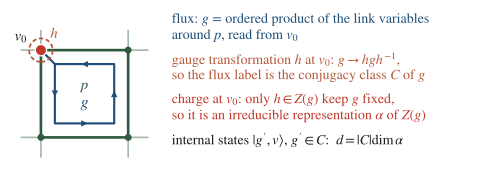
Figure 2. A flux–charge composite of $D(G)$. The flux is a holonomy measured from a base point, the gauge freedom at the base point reduces it to a conjugacy class, and only the centralizer survives to act on the charge. The holonomy is read counterclockwise from $v_0$, the plaquette orientation of conventions §1.

7.3 The count for $S_3$ [Computed.]

$S_3$ has the classes $\{e\}$ ($|C|=1$, $Z=S_3$), the three transpositions ($|C|=3$, $Z={\mathbb{Z}}_2$) and the two 3-cycles ($|C|=2$, $Z={\mathbb{Z}}_3$). $S_3$ has three irreducible representations (trivial, sign, the 2-dimensional standard one), ${\mathbb{Z}}_2$ two and ${\mathbb{Z}}_3$ three, with ${\chi }_j((123))={\omega }^j$:

anyon	$A$	$B$	$C$	$D$	$E$	$F$	$G$	$H$
flux class	$e$	$e$	$e$	$(12)$	$(12)$	$(123)$	$(123)$	$(123)$
charge	trivial	sign	standard	$+$	$-$	$1$	$\omega$	$\bar{\omega }$
$d$	1	1	2	3	3	2	2	2
$\theta$	1	1	1	1	$-1$	1	$\omega$	$\bar{\omega }$

Table 1. The eight anyons of $D(S_3)$, with $d$ from (7.1) and θ from (7.4).

Then ${\mathcal{D}}^2=1+1+4+9+9+4+4+4=36$ and $\mathcal{D}=6=|S_3|$, as (7.2) requires. The anyons $D$ and $E$, with $d=3$, are the transposition fluxes. The charges $\omega$, $\bar{\omega }$ bound to a 3-cycle are not representations of $S_3$; a free doublet $C$ next to the flux splits into them, $C\times F=G+H$ (§7.4). By enumeration, $S_3$ has 18 commuting pairs, which fall into 8 orbits under simultaneous conjugation, and 48 commuting triples, so $Z(T^3)=48/6=8$, in agreement with (7.3) and with $Z(T^2\times S^1)=\mathrm{GSD}(T^2)$.

7.4 Modular data and non-abelian braiding [Stated — refs: Coste–Gannon–Ruelle, up to the conjugation convention; checked numerically.]

For anyons $(A,\alpha )$ and $(B,\beta )$, choose $x_g$ with $x_g{g}_A{x}_g^{-1}=g$ for every $g\in A$, and similarly $y_h$ for $h\in B$. Then

$$S_{(A,\alpha ),(B,\beta )}=\frac{1}{|G|}\sum _{\begin{array}{c}g\in A,h\in B\\ gh=hg\end{array}}{\chi }_{\alpha }\left(x_g^{-1}h{x}_g{)}^{\ast }{\chi }_{\beta }\right(y_h^{-1}g{y}_h{)}^{\ast }.\text{\hspace{1em}(7.5)}$$

For $S_3$, in the order of Table 1, (7.5) gives a real matrix,

$$S=\frac{1}{6}\left(\begin{array}{cccccccc}1& 1& 2& 3& 3& 2& 2& 2\\ 1& 1& 2& -3& -3& 2& 2& 2\\ 2& 2& 4& 0& 0& -2& -2& -2\\ 3& -3& 0& 3& -3& 0& 0& 0\\ 3& -3& 0& -3& 3& 0& 0& 0\\ 2& 2& -2& 0& 0& 4& -2& -2\\ 2& 2& -2& 0& 0& -2& -2& 4\\ 2& 2& -2& 0& 0& -2& 4& -2\end{array}\right),T=\mathrm{diag}(1,1,1,1,-1,1,\omega ,\bar{\omega }).\text{\hspace{1em}(7.6)}$$

We checked that $S$ is symmetric and orthogonal with $S^2=1$ (every anyon is self-dual), that $(ST{)}^3=S^2$ with $\Theta =1$, so $c\equiv 0$ mod 8, that $S_{0a}/S_{00}$ reproduces the $d$ of Table 1, that the Verlinde formula gives non-negative integers, and that (6.1) rebuilt from those fusion rules and the spins (7.4) returns (7.5). For $G={\mathbb{Z}}_2$, (7.5) gives $S_{\mathrm{TC}}$. Among the fusion rules,

$$D\times D=A+C+F+G+H,G\times G=A+B+G,G\times H=C+F,$$

and the space of four $D$‘s with total charge $A$ has dimension ${\sum }_c(N_{DD}^c{)}^2=5$. Braiding acts on such multidimensional fusion spaces by matrices: these anyons are non-abelian. A one-number diagnostic is the monodromy scalar $M_{ab}=S_{ab}^{\ast }{S}_{00}/(S_{0a}{S}_{0b})$, which for abelian anyons is the braiding phase $B(a,b)$, the monodromy of Weeks 7–8, of modulus one; for the charge $C$ and the flux $F$, $M_{CF}=\frac{(-2/6)(1/6)}{(2/6)(2/6)}=-\frac{1}{2}$, which is ${\chi }_C((123))/2$.

Physical picture. The number $-\frac{1}{2}$ is the normalized trace of the matrix that the standard representation assigns to a 3-cycle, a rotation by $2\pi /3$. A doublet charge carried around a 3-cycle flux comes back rotated in its internal space, and an interferometer comparing the encircling and the direct paths sees the overlap $-\frac{1}{2}$, of modulus less than one: the non-abelian Aharonov–Bohm effect, exact in the quantum double. Around a transposition flux the overlap is ${\chi }_C((12))/2=0$. A flux is itself conjugated by the holonomy it encircles, so the braiding of several fluxes acts on their fusion space [Heuristic reading of (7.5)].

8. The edge: chiral bosons and the bulk–edge correspondence

8.1 The edge action [Computed; the velocity term Sketched — refs: Wen, PRB 41 (1990) 12838.]

Put the fluid in the region $y\le 0$ with its edge at $y=0$ (Figure 3). In the gauge $a_t=0$ the constraint $f=0$ makes $a_i^I={\partial }_i{\varphi }^I$ in the bulk, with ${\varphi }^I$ compact. The kinetic term of (2.2) becomes

$$\frac{1}{4\pi }{K}_{IJ}({\partial }_y{\varphi }^I{\partial }_x{\dot{\varphi }}^J-{\partial }_x{\varphi }^I{\partial }_y{\dot{\varphi }}^J)=\frac{1}{4\pi }{K}_{IJ}\left[{\partial }_y\right({\varphi }^I{\partial }_x{\dot{\varphi }}^J)-{\partial }_x({\varphi }^I{\partial }_y{\dot{\varphi }}^J\left)\right],$$

a total derivative. The ${\partial }_x$ term integrates to zero along the edge, and the ${\partial }_y$ term leaves, after an integration by parts in $x$ with $K$ symmetric,

$$S_{\mathrm{edge}}=-\frac{1}{4\pi }\int dtdx{K}_{IJ}{\partial }_x{\varphi }^I{\partial }_t{\varphi }^J.\text{\hspace{1em}(8.1)}$$

The boundary condition that makes the edge dynamics well posed is set by the confining potential and is not universal; it adds a Hamiltonian $\frac{1}{4\pi }\int dx{V}_{IJ}{\partial }_x{\varphi }^I{\partial }_x{\varphi }^J$ with $V$ positive definite, and

$$S_{\mathrm{edge}}=-\frac{1}{4\pi }\int dtdx[K_{IJ}{\partial }_t{\varphi }^I{\partial }_x{\varphi }^J+V_{IJ}{\partial }_x{\varphi }^I{\partial }_x{\varphi }^J],\text{\hspace{1em}(8.2)}$$

the multicomponent chiral boson.

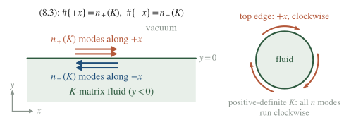
Figure 3. The edge of a $K$-matrix fluid. By (8.3) the number of modes moving in $+x$ is the number of positive eigenvalues of $K$; along the top of the fluid $+x$ is the clockwise sense.

8.2 Chirality, the edge algebra and the correspondence [Proved for (8.3); (8.4)–(8.5) Computed; the correspondence Stated — refs: Wen 1990; Witten 1989.]

The equation of motion of (8.2) is ${\partial }_x(K{\partial }_t\varphi +V{\partial }_x\varphi )=0$, and a mode $\varphi \propto {\varphi }_0{e}^{iq(x-vt)}$ requires $vK{\varphi }_0=V{\varphi }_0$. The velocities are the eigenvalues of $K^{-1}V$, which is similar to $V^{1/2}{K}^{-1}{V}^{1/2}$, a matrix congruent to $K^{-1}$. By Sylvester’s law of inertia,

$$\#\{\text{modes moving in }+x\}=n_{+}(K),\#\{\text{modes moving in }-x\}=n_{-}(K),\text{\hspace{1em}(8.3)}$$

independently of $V$ (checked with random positive $V$ for five matrices). Along the top edge of the fluid, $+x$ is clockwise, so $\sigma (K)$ net modes run clockwise: $c=-\sigma (K)$ counterclockwise, as (6.4) found modulo 8. The first-order term of (8.2) is $\frac{1}{2}\int \varphi J\dot{\varphi }$ with $J=\frac{K}{2\pi }{\partial }_x$; the bracket is the inverse kernel, $2\pi K^{-1}\cdot \frac{1}{2}\mathrm{sgn}(x-y)$, so

$$[{\varphi }^I(x),{\varphi }^J(y)]=i\pi (K^{-1}{)}^{IJ}\mathrm{sgn}(x-y),\text{\hspace{1em}(8.4)}$$

which we checked against the mode sum of a single field on a circle. For the vertex operators $V_l=e^{il\cdot \varphi }$,

$$V_l(x)V_{l^{\prime }}(y)=e^{-i\pi l^T{K}^{-1}{l}^{\prime }\mathrm{sgn}(x-y)}{V}_{l^{\prime }}(y)V_l(x),\text{\hspace{1em}(8.5)}$$

the exchange phases of (4.3) on the edge. The electron $V_{Kt}$ obeys $V_{Kt}(x)V_{Kt}(y)=(-1{)}^{t^{T}Kt}{V}_{Kt}(y)V_{Kt}(x)$, a fermion for $K=3$, and the local operators $V_{Kv}$ have trivial full braiding with every $V_l$.

The bulk–edge correspondence states that the edge of the theory (2.1) is the chiral boson (8.2), with chiral central charge $c=-\sigma (K)$ counted counterclockwise and primary fields labelled by $\mathcal{A}$, whose conformal spins $\frac{1}{2}{l}^T{K}^{-1}l$ mod 1 are the bulk spins measured in the sense of propagation; the edge of a chiral theory cannot be gapped. For $\nu =1/3$ there is one clockwise mode, the quasiparticle operator $e^{i\varphi }$ has conformal spin $\frac{1}{6}$ and the electron $e^{3i\varphi }$ has $\frac{3}{2}$. For the toric code there is one mode each way, and Problem 8⋆ gaps them.

9. Seminar: Wen–Niu, degeneracy on high-genus surfaces

Format. As in syllabus §7: the presenter states the technical claim, identifies what it needs from Semester I and reproduces one step at the board; discussion follows, and the instructor places the result on the course map. Every student reads the assigned parts and brings Problem 1.

Parts. The torus degeneracy of the $\nu =1/q$ state from the Wilson-loop algebra of its effective $U(1)$ Chern–Simons theory, its extension to genus $g$, its relation to the quasiparticle statistics, and the splitting estimate; the Ginzburg–Landau duality is optional.

The technical claim. Fractional quantum Hall states have ${\tilde{q}}^g$ ground states on a surface of genus $g$, $\tilde{q}$ being the torus degeneracy, tied to the quasiparticle statistics $\theta =\tilde{p}\pi /\tilde{q}$; the degeneracy survives weak arbitrary perturbations, it is split by at most $e^{-L/\xi }$ in a system of size $L$, and phases with different degeneracies have different topological orders.

What it needs from Semester I. The Chern–Simons term as a Hall response (Sem I Week 12 §8.2); the Gauss law and the Hamiltonian Hilbert space of a gauge theory (Sem I Week 7); and from this semester the holonomy algebra of Week 2 §§3–4.

The step at the board. The mini-step of the week: GSD, spins and mutual statistics from the $K$-matrix for $\nu =1/3$ and for the toric code, matched to Week 8. In twenty minutes, (3.1)–(3.4) at $K=3$, then (4.1) and (4.3), then §5.2 with the labels of Week 8; in ten, the comparison with Wen and Niu’s $q^g$.

For the discussion. Week 9 traces the robustness of the degeneracy to the code distance: compare that argument with Wen and Niu’s, and ask what the electron’s sign (F2) changes on the torus.

The open question it leaves for this course. The lattice models of Weeks 8 and 11 are non-chiral sums of commuting projectors; a lattice model of a chiral $K$, or a lattice Chern–Simons term built with the cup products of conventions §8, is the open question.

On the course map. The Laughlin state is the chiral relative of the BF theory of Week 2, and its response (4.5) is the Chern–Simons layer of the θ-wall of Sem I Week 12.

10. Subtleties and fine print

F1. The global definition of the action. The $S^1\times \Sigma$ argument of Week 2 (2.2) gives different answers for $b\wedge da$ and $\frac{1}{2}(a\wedge db+b\wedge da)$, which differ by $d(a\wedge b)$, a term that fails to be gauge invariant when fluxes are present. The 4-manifold definition of §2.1 removes the ambiguity and gives the parity of $K_{II}$ its meaning (Week 2 §9.1 for BF).

F2. Fermionic $K$. For odd $K_{II}$ the theory needs a spin structure: the local fermion $K{e}_I$ has $\theta =-1$, anyon spins are defined modulo its sign, a line $W_{Kv}(\gamma )$ with odd $v^{T}Kv$ acts on a cycle by the sign that the spin structure assigns to it, and the modular relations involve $T^2$ [Stated]. The degeneracy $|\det K|$ holds for each spin structure; the Laughlin states at $\nu =1/3$ and $1/5$ are of this kind.

F3. Equivalent $K$. For $W\in GL(n,\mathbb{Z})$ the change of variables $a\to Wa$ maps $(K,t)$ to $(W^{T}KW,W^{T}t)$ and the quasiparticle labels as $l\to W^{T}l$; the data $(\mathcal{A},\theta ,B,\sigma ,\nu )$ are invariant. The double semion appears as $\mathrm{diag}(2,-2)$ and as $\left(\begin{array}{cc}2& 2\\ 2& 0\end{array}\right)$ (Problem 6⋆), and stacking with the trivial theory $\left(\begin{array}{cc}0& 1\\ 1& 0\end{array}\right)$ changes no datum.

F4. Spin and exchange. For abelian anyons the spin equals the exchange phase. For non-abelian anyons θ is the phase of a $2\pi$ rotation of one anyon, (7.4), while the exchange of two anyons depends on their fusion channel; (7.6) records the former.

F5. The orientation is part of the data. Reversing the orientation of $M$ sends $K\to -K$, $\theta \to {\theta }^{\ast }$, $S\to S^{\ast }$ and $c\to -c$, so a table of spins without its orientation convention is ambiguous for chiral theories; for $\nu =1/3$ the mirror theory has the opposite Hall sign and edge direction (§4.4).

11. Common misconceptions

”$|\det K|=1$ means a trivial phase.” It is tempting because there are no anyons and the torus has one state. A unimodular $K$ with $\sigma (K)\ne 0$ has chiral edge modes by (8.3), and for $K=1$ a Hall response, (4.6): it is an invertible phase with a protected edge.

“Anyons of $D(G)$ are a conjugacy class and an irreducible representation of $G$.” It is tempting because pure charges are irreducible representations of $G$. A charge bound to a flux $g$ transforms under $Z(g)$ only; for $S_3$ this gives 8 anyons, against 9 from the wrong rule, and charges ω, $\bar{\omega }$ that no free charge carries.

12. Historical note

Laughlin (1983) proposed the wave function of the $\nu =1/m$ state, analyzed it through its analogy with a two-dimensional plasma, and found quasiholes of charge $e/m$ by inserting a flux quantum. Arovas, Schrieffer and Wilczek (1984) computed the Berry phase of a quasihole carried around a closed path and identified its fractional statistics. Witten (1989) built the topological field theory of the Chern–Simons action, computed its Wilson loops, including the linking numbers of the abelian theory and their framing dependence, and identified its Hilbert spaces with the conformal blocks of the WZW model. Wen and Niu (1990) derived the $q^g$ degeneracy from the effective Chern–Simons theory and proposed it as the defining quantum number of topological order, and in the same year Wen derived the chiral Luttinger-liquid theory of the edge. Wen and Zee (1992) organized the abelian quantum Hall states by an integer matrix $K$ and a charge vector $t$. Kitaev’s 1997 preprint built lattice Hamiltonians for any finite group whose anyons realize the quantum double, and Coste, Gannon and Ruelle (2000) worked out the modular data of the (twisted) doubles of finite groups.

13. What to take away

1. Technical: the bracket (2.3) gives the holonomy algebra (2.5) and $\mathrm{GSD}({\Sigma }_g)=|\det K{|}^g$. Physical: the degeneracy counts the anyon types $\mathcal{A}={\mathbb{Z}}^n/K{\mathbb{Z}}^n$, one state per type on the torus.
2. Technical: each quasiparticle carries the flux $-2\pi K^{-1}l$, so $B(l,l^{\prime })=e^{-2\pi i{l}^T{K}^{-1}{l}^{\prime }}$, ${\theta }_l=e^{-i\pi l^T{K}^{-1}l}$ counterclockwise, $Q_l=-t^T{K}^{-1}l$ and ${\sigma }_{xy}=-\nu e^2/2\pi$. Physical: every topological number is an Aharonov–Bohm phase of a charge–flux composite; $K=3$ gives charge $e/3$, angle $\pi /3$ and three states.
3. Technical: $S$ and $T$ of (6.1) satisfy (6.2); for $K$-matrices they are (6.3), with $\Theta =e^{-2\pi i\sigma (K)/8}$. Physical: the modular data are the fingerprint; they separate the toric code from the double semion and fix $c$ mod 8.
4. Technical: $D(G)$ anyons are pairs (class, irreducible representation of the centralizer), with $d=|C|\dim \alpha$ and $\mathcal{D}=|G|$; $D(S_3)$ has 8 anyons with $d=1,1,2,3,3,2,2,2$. Physical: non-abelian gauge groups give non-abelian anyons, whose braiding acts by matrices on fusion spaces.
5. Technical: the edge is the chiral boson (8.2), with $n_{\pm }(K)$ modes in the two directions. Physical: chirality is a bulk invariant that a heat or charge current along the edge measures.

14. Looking ahead

Week 11 builds topological orders as condensates of string nets (string-net-condensation): the toric code and the double semion reappear as the two ${\mathbb{Z}}_2$ string nets, and the input data are the $F$-symbols of Week 7, now the weights of a wave function. String-net models are non-chiral, $\Theta =1$, the lattice face of the open question of §9. Block 5 returns to condensation: condensing a bosonic anyon subgroup, as Problem 9⋆⋆ does for $D({\mathbb{Z}}_N)$, is the topological-order form of Higgsing and of the gapped edges of Problem 8⋆, and leads to the condensation-defects of the group’s research line (forward references).

15. Problem set

Problems 1–4 are the classroom core; 5⋆–8⋆ consolidate the self-study sections; 9⋆⋆–10⋆⋆ are research extensions.

Core problems

1. The $\nu =2/5$ and $\nu =1/5$ states (extends §§3, 4, 5.1, 8.2). Take $K=\left(\begin{array}{cc}3& 2\\ 2& 3\end{array}\right)$ and $t=(1,1)$. (a) Compute $\det K$, $\mathcal{A}$ and $\mathrm{GSD}({\Sigma }_g)$, and show that $(1,0)$ and $(0,1)$ are the same anyon. (b) Compute ν and ${\sigma }_{xy}$. (c) Find the charge and the statistics angle of $l=(1,0)$, and decide whether $(1,-1)$ is a local excitation. (d) How many edge modes are there, and in which sense do they run? (e) Repeat (b)–(c) for $K=5$, $l=1$.

2. $D({\mathbb{Z}}_N)$ from $K=\left(\begin{array}{cc}0& N\\ N& 0\end{array}\right)$ (extends §§5.2, 6.2). (a) From (4.3) with $l=(a,-b)$, compute the braiding $B(e^a{m}^b,e^{a^{\prime }}{m}^{b^{\prime }})$ of two general dyons and read it as Aharonov–Bohm phases of each charge in the other’s flux. (b) Show $S_{(a,b),(a^{\prime },b^{\prime })}=\frac{1}{N}{\omega }^{-(a{b}^{\prime }+a^{\prime }b)}$ and $S^2=C$ with $C:(a,b)\to (-a,-b)$. (c) Compute Θ. (d) For $N=3$, list the bosons.

3. The semion and the edge sense (extends §§6.2, 8.2). Take $K=2$. (a) Find $\mathcal{A}$, the spins, $S$ and $T$. (b) Verify $(ST{)}^3=\Theta S^2$ by multiplying the matrices and find Θ. (c) Read $c$ from Θ and compare with the direction of the edge mode given by (8.3).

4. Fusion and monodromy in $D(S_3)$ (extends §7.4). (a) From (7.6), compute $C\times C$, $C\times F$ and $F\times F$ with the Verlinde formula, and check $d_a{d}_b={\sum }_c{N}_{ab}^c{d}_c$ in each case. (b) Compute the monodromy scalars $M_{CF}$ and $M_{CD}$ and compare them with ${\chi }_C(g)/2$ for the corresponding fluxes. (c) What is the dimension of the space of four $F$ anyons with total charge $A$?

Starred problems

5⋆. The Halperin $(3,3,1)$ state and the Smith form (extends §§2.3, 4.3). For $K=\left(\begin{array}{cc}3& 1\\ 1& 3\end{array}\right)$, $t=(1,1)$: show that $\mathcal{A}\cong {\mathbb{Z}}_8$ and not ${\mathbb{Z}}_2\times {\mathbb{Z}}_4$, compute ν and the charge and spin of $(1,0)$, and decide whether $(1,0)$ and $(0,1)$ are the same anyon. Hint: $K^{-1}(1,0{)}^T=(\frac{3}{8},-\frac{1}{8})$ has order 8 in $(\mathbb{Q}/\mathbb{Z}{)}^2$; for the last part test whether $K^{-1}(1,-1{)}^T$ is integral.

6⋆. Twisted ${\mathbb{Z}}_N$ doubles as $K$-matrices (extends §5.3 and Week 7 Problem 6⋆). Show that $K=\left(\begin{array}{cc}2k& N\\ N& 0\end{array}\right)$ with the label $l=(-n,x)$ reproduces ${\theta }_{(x,n)}=\exp (2\pi i(\frac{xn}{N}+\frac{k{x}^2}{N^2}))$ of Week 7 Problem 6⋆, and for $N=2$, $k=1$ find $W\in GL(2,\mathbb{Z})$ with $W^{T}KW=\mathrm{diag}(2,-2)$; which label is $s$? Hint: $K^{-1}=\left(\begin{array}{cc}0& 1/N\\ 1/N& -2k/N^2\end{array}\right)$; for $W$, complete the square in $2v_1^2+4v_1{v}_2$.

7⋆. $D(D_4)$ and $D(Q_8)$ (extends §7.2). Count the anyons of both doubles, compute $\mathcal{D}$ and the multiset of quantum dimensions, and show that the multisets of spins differ. Hint: in $D_4$ the rotation of order 4 has centralizer ${\mathbb{Z}}_4$ and each reflection ${\mathbb{Z}}_2\times {\mathbb{Z}}_2$; in $Q_8$ every non-central element has centralizer ${\mathbb{Z}}_4$; at the central element of order 2 the two-dimensional irreducible representation is $-1$.

8⋆. Gapping the toric-code edge (extends §8.2). For $K=\left(\begin{array}{cc}0& 2\\ 2& 0\end{array}\right)$, show that $V_{(2,0)}$ is local and that (8.4) gives $[{\varphi }^1(x),{\varphi }^1(y)]=0$; argue that $-g\int \cos (2{\varphi }^1)$ pins ${\varphi }^1$ and gaps both edge modes, and identify the anyon whose edge operator acquires an expectation value. Show that for $K=2$ no nonzero local $l$ has $l^T{K}^{-1}l=0$. Hint: $(K^{-1}{)}^{11}=0$; a field that commutes with itself at all separations can be pinned classically.

⋆⋆ problems

9⋆⋆. Anyon condensation as Higgsing. Known: the condensation rules of Week 8 §7.5; in $D({\mathbb{Z}}_N)$ the charge $e^q$, $q\mid N$, is a boson with trivial self-braiding; charge-$q$ matter leaves the residual ${\mathbb{Z}}_{\gcd (N,q)}^{(1)}$ of conventions §6 (Sem II Week 3; subgroup gauging in Sem II Week 4); the group’s charge-$k$ condensate realizes subgroup higher gauging (julia-toulouse-mechanism, Block 5). Explored: condense $L=⟨e^q⟩$ by keeping the anyons that braid trivially with $L$ and identifying them modulo $L$, $L^{\perp }/L$; show that the result has the modular data of $K^{\prime }=\left(\begin{array}{cc}0& q\\ q& 0\end{array}\right)$, with the flux $m^{N/q}$ as its elementary flux. Sources: §§4–6 and the notes cited. Completion: a proof for general $N$ and $q\mid N$ with $S$ and $T$ of $L^{\perp }/L$ computed and matched to (6.3) for $K^{\prime }$, a numerical check for $N\le 12$, and one page relating the condensed anyons to the condensation wall of the group’s manuscript.

10⋆⋆. Braiding of transposition fluxes in $D(S_3)$. Known: §7.4; the flux conjugation rule (in one convention an exchange maps a pair of fluxes $(g,h)$ to $(gh{g}^{-1},g)$); the Verlinde count $\dim V(D,D,D,D\to A)=5$. Explored: the action of the braid group on four transposition fluxes with trivial total flux and trivial charges, modulo global conjugation. Sources: §§7.2–7.4, the Verlinde formula (6.2), and Kitaev, quant-ph/9707021, §6, “Topological operators, braiding, and fusion” (arXiv numbering; §7 in the Annals version). Completion: the Burnside count of the 27 flux configurations, 5 orbits, matching the Verlinde count; the $5\times 5$ permutation matrices of the three braid generators with the exchange rule stated; the braid relations checked numerically; and the order of the finite group they generate.

Self-study answer checkpoints

Problem 1. Decisive step: $K^{-1}=\frac{1}{5}\left(\begin{array}{cc}3& -2\\ -2& 3\end{array}\right)$, and $(1,-1)=K(1,-1{)}^T$ lies in $K{\mathbb{Z}}^2$. Result: $\det K=5$, $\mathcal{A}={\mathbb{Z}}_5$, $\mathrm{GSD}=5^g$; $(1,0)-(0,1)=(1,-1)$ is local, so the two labels coincide; $\nu =\frac{2}{5}$, ${\sigma }_{xy}=-\frac{2}{5}{e}^2/2\pi$; $Q_{(1,0)}=-\frac{1}{5}$ and $l^T{K}^{-1}l=\frac{3}{5}$, so ${\theta }_{(1,0)}=e^{-3\pi i/5}$, statistics angle $\frac{3\pi }{5}$; $(1,-1)$ is a neutral local boson ($l^T{K}^{-1}l=2$); two modes, both clockwise ($n_{+}=2$). For $K=5$: $Q=-\frac{1}{5}$, $\theta =e^{-i\pi /5}$, ${\sigma }_{xy}=-\frac{1}{5}{e}^2/2\pi$. Common failure: treating $\mathcal{A}$ as ${\mathbb{Z}}_5\times {\mathbb{Z}}_5$, or quoting $\theta =e^{+3\pi i/5}$ counterclockwise with the weight (2.1).

Problem 2. Decisive step: $l^T{K}^{-1}{l}^{\prime }=-(a{b}^{\prime }+a^{\prime }b)/N$ for $l=(a,-b)$, $l^{\prime }=(a^{\prime },-b^{\prime })$. Result: $B(e^a{m}^b,e^{a^{\prime }}{m}^{b^{\prime }})={\omega }^{a{b}^{\prime }+a^{\prime }b}$, the phase ${\omega }^{a{b}^{\prime }}$ of charge $a$ in flux $b^{\prime }$ times ${\omega }^{a^{\prime }b}$ of charge $a^{\prime }$ in flux $b$, equal to ${\theta }_{l+l^{\prime }}/({\theta }_l{\theta }_{l^{\prime }})$ with $\theta ={\omega }^{ab}$; $S$ as stated, and $(S^2{)}_{(a,b),(a^{\prime \prime },b^{\prime \prime })}={\delta }_{a,-a^{\prime \prime }}{\delta }_{b,-b^{\prime \prime }}$ by summing the geometric series; $\Theta =\frac{1}{N}{\sum }_{a,b}{\omega }^{ab}=1$, since ${\sum }_b{\omega }^{ab}=N{\delta }_{a,0}$. For $N=3$ the bosons are $1,e,e^2,m,m^2$. Common failure: labelling $m=(0,1)$, which inverts every braiding phase relative to conventions §9, or normalizing Θ by ${\mathcal{D}}^2=N^2$.

Problem 3. Decisive step: $T=\mathrm{diag}(1,e^{-i\pi /2})$ from (6.3). Result: $\mathcal{A}={\mathbb{Z}}_2$, $\theta =(1,-i)$, $S=\frac{1}{\sqrt{2}}\left(\begin{array}{cc}1& 1\\ 1& -1\end{array}\right)$, $S^2=1$; $(ST{)}^3=e^{-i\pi /4}1$, so $\Theta =\frac{1-i}{\sqrt{2}}=e^{-2\pi i/8}$ and $c\equiv -1$; (8.3) gives one mode along $+x$, clockwise, which is $c=-1$ counterclockwise. Common failure: taking $\theta =+i$ with the weight (2.1), which gives $c=+1$ and the wrong edge direction, or normalizing Θ by ${\mathcal{D}}^2=2$.

Problem 4. Decisive step: $N_{ab}^c={\sum }_x{S}_{ax}{S}_{bx}{S}_{cx}/S_{0x}$ with the real $S$ of (7.6) and $S_{0x}=d_x/6$. Result: $C\times C=A+B+C$ ($4=1+1+2$), $C\times F=G+H$ ($4=2+2$), $F\times F=A+B+F$ ($4=1+1+2$); $M_{CF}=-\frac{1}{2}={\chi }_C((123))/2$ and $M_{CD}=0={\chi }_C((12))/2$; four $F$‘s with total charge $A$ span ${\sum }_c(N_{FF}^c{)}^2=3$ states. Common failure: dividing by $S_{00}$ in place of $S_{0x}$ in the Verlinde sum, which gives non-integer coefficients.

---

Notes prepared for the generalized-symmetries course, Semester II Block 3. Written to the note-quality-template standard on 2026-10-02. Last revised 2026-10-04.