Sem II Week 4 — Gauging: Backgrounds, Orbifolds and the Quantum Dual Symmetry

Every duality of Semester I ended with a sum over boundary-condition sectors. This week we name that sum. We carry this out operator by operator on the transverse-field Ising chain, where the new symmetry is the holonomy of the new gauge field and the Kramers–Wannier operator of Week 4 becomes an explicit composite of gauging maps; we then derive the degree rule by counting backgrounds, gauge subgroups with the annihilator bookkeeping of Week 14, and read the difference between $SU(N)$ and $SU(N)/{\mathbb{Z}}_N$ off a ${\mathbb{Z}}_N$ lattice toy. Mini-calculation 1 repeats the construction one dimension up. Block 1 closes here, and Block 2 asks what happens when the sum over backgrounds cannot be defined.

How to use this chapter

• In class: in the first lecture derive the coupling to backgrounds and the normalization (2.5) (§§2.1–2.2), then the gauged chain in the order of §3: the Gauss law (3.2), the cocycle sum (3.4), the dual variables (3.6), the orbifold Hilbert space (3.7), the dual symmetry (3.8)–(3.11), and the Kramers–Wannier operator as a composite of gauging maps, (3.12), with the three-site matrices of §3.7 on the board. Problems 1 and 2 belong to this lecture. In the second lecture derive the degree rule and its inverse (§§4.1–4.3), the torus form of Kramers–Wannier as gauging (§4.4), the gauged exact sequence (§5.1) and the lattice toy of §6.1, and state the continuum classification of §6.2; Problems 3 and 4. The seminar hour (§8) is Aharony–Seiberg–Tachikawa.
• For self-study: the general-degree normalization of §2.2, the fractional residual charge of §5.2, the classification proof of §6.2, §§9–10 and Problems 5⋆–7⋆. Mini-calculation 1 (§7) is handed in at the end of the week; the one calculation to do alone is its Sub-task 1, the four-site chain with every matrix written out.
• Instructor checkpoint: two errors recur. The first is to treat gauging as a projection onto invariant states: Gauss’s law does project onto $\eta =1$, but the sum over link configurations adds the twisted sector, and the gauged chain has $2^L$ states, twice the number of invariant states of the periodic chain (§3.4). The second concerns pairings and shifts. The dual background enters through the cup product, which on the torus pairs the two sector labels crosswise, ${ϵ}_1{c}_2+{ϵ}_2{c}_1$, and the dot pairing $ϵ\cdot c$ fails on every non-square torus (§4.4); likewise the half-site shift in the Kramers–Wannier operator is what puts $T$, and not $T^{-1}$, into $D^2=(1+\eta )T$ (§3.6).

0. Reading

Primary: Gaiotto, Kapustin, Seiberg, Willett (GKSW), “Generalized global symmetries”, JHEP 02 (2015) 172 [arXiv:1412.5148], §3, pp. 11–12 (the paragraph on twisted-sector operators, the quantum $(d-q-2)$-form symmetry and the inequivalent ways of gauging), and §4.3, pp. 16–18. Aharony, Seiberg, Tachikawa (AST), “Reading between the lines of four-dimensional gauge theories”, JHEP 08 (2013) 115 [arXiv:1305.0318], §§1.1–1.3 (pp. 2–6), 2.1 (pp. 11–12), 2.3 (pp. 13–14) and 6.4 (from p. 36): the seminar paper of §8.

Secondary: Kapustin & Seiberg, arXiv:1401.0740, §§1–3, on coupling a theory to a discrete gauge theory; Week 4 §§3.4 and 4.4, Week 5 §§7–8, Week 14 §§3, 6–7 and Week 15 §§2 and 3.4, whose sector sums and exact sequence this week reorganizes; Sem II Week 1 §5 (the linking action on the lattice) and Sem II Week 2 §6 (the cup product and the lattice dictionary); McGreevy, arXiv:2204.03045, for gauging in lattice language.

Optional research reading: Tachikawa, “On gauging finite subgroups”, SciPost Phys. 8 (2020) 015 [arXiv:1712.09542], on the symmetry of a theory in which a normal abelian subgroup has been gauged (§5); Vafa, “Quantum symmetries of string vacua”, Mod. Phys. Lett. A 4 (1989) 1615, where the name comes from (§11); GKSW §§4.2 and 5.3–5.4 on $SU(N)$ and $PSU(N)$.

Proof-status labels as in Week 1. Every sign and normalization is from conventions and every degree from its §6. The normalization (2.4)–(2.5) of the sum over backgrounds and the signs of the dual coupling and of its inverse, (4.1) and (4.3), are recorded in conventions §6; the closed form (3.12) of the Kramers–Wannier operator, the link qubits, the Gauss operators and the chain length $L$ are recorded in its §4.

1. Motivation and setting

Semester I gauged in two senses. In Week 5 Wegner made the Ising flip local by introducing link variables, and gave them a plaquette action of their own, which produced a new dynamical theory. Elsewhere the course summed over sectors without calling it gauging. The four boundary-condition sectors of the 2d Ising model enter the torus form of Kramers–Wannier duality with the intersection form as a sign (Sem I Week 4 §3.4); the eight sectors of the 3d Ising model are summed in the torus form of Wegner’s duality (conventions §4); and ‘t Hooft’s twisted boundary conditions label the magnetic flux sectors of ${\mathbb{Z}}_N$ gauge theory (Sem I Week 14 §6.2). Week 15 §2 recorded that a symmetry operator on a noncontractible cycle is a twisted boundary condition, and postponed the rest to this week.

The physical question is this. Given a theory $T$ with a discrete symmetry, we want a new theory $T/G$ in which the symmetry has become a redundancy, and we want its partition function, its Hilbert space, its operators and its symmetries. Three answers organize the week. The new theory is defined by a normalized sum over flat backgrounds, so that its torus partition function is a finite combination of twisted partition functions of $T$ (§2). Its Hilbert space on a circle is the symmetric part of every twisted sector of $T$, and its operators are the neutral operators of $T$ together with the endpoints of the symmetry operators of $T$, which become genuine local or extended operators (§3). And it carries a new symmetry, the quantum dual symmetry, which is in general one of the higher-form-symmetries, of degree $d-p-2$ (§4). For $p=0$ and $d=2$ the dual symmetry is a ${\mathbb{Z}}_2^{(0)}$, and the identification of $T/{\mathbb{Z}}_2$ with $T$ at the dual coupling is kramers-wannier-duality. Gauging a subgroup (§5) and gauging part of the center of a gauge group (§6) are the same construction with the bookkeeping of Sem I Week 14 §3.

2. Backgrounds and the sum over cocycles

2.1 Coupling a ${\mathbb{Z}}_N^{(p)}$ symmetry to a background [Proved.]

The lattice models of the course with a discrete $p$-form symmetry share one structure. Let $X$ be a closed oriented cell complex of dimension $d$ (in practice the hypercubic torus of conventions §1), let the field be $\varphi \in C^p(X,{\mathbb{Z}}_N)$, and let the weight be a product over the $(p+1)$-cells $c$,

$$Z_T=\sum _{\varphi \in C^p(X,{\mathbb{Z}}_N)}\prod _{c}w((d\varphi {)}_c),\text{\hspace{1em}(2.1)}$$

where $w$ is a positive function on ${\mathbb{Z}}_N$. For $p=0$ this is a clock model, with $w(n)=e^{K\cos (2\pi n/N)}$ and the Ising model at $N=2$; for $p=1$ it is ${\mathbb{Z}}_N$ gauge theory, with $w(n)=e^{\beta \cos (2\pi n/N)}$ and Wegner’s model at $N=2$ (conventions §4). The shift $\varphi \to \varphi +\epsilon$ with $d\epsilon =0$ leaves every factor unchanged. For $p=0$ the closed $\epsilon$ are the constants, the global ${\mathbb{Z}}_N^{(0)}$; for $p=1$ they are the flat cochains, which act on Wilson loops through their holonomies, the electric ${\mathbb{Z}}_N^{(1)}$ of conventions §6. Exact shifts are gauge transformations for $p=1$, so the symmetry acting on the torus is $H^p(X,{\mathbb{Z}}_N)$.

Couple to a background $B\in C^{p+1}(X,{\mathbb{Z}}_N)$ by

$$Z_T[B]=\sum _{\varphi }\prod _{c}w((d\varphi -B{)}_c).\text{\hspace{1em}(2.2)}$$

For every $\lambda \in C^p(X,{\mathbb{Z}}_N)$ the change of variables $\varphi \to \varphi +\lambda$ maps the summand at $B$ to the summand at $B+d\lambda$, so

$$Z_T[B+d\lambda ]=Z_T[B].\text{\hspace{1em}(2.3)}$$

A background is a configuration of symmetry defects. For $p=0$, $d=2$, $N=2$, the closed cochain $a$ that equals 1 on the horizontal links crossed by one vertical dual cycle flips exactly those bonds: it is the seam of Sem I Week 4 §3.4, and the label ${ϵ}_1$ there is the holonomy of $a$ along the horizontal cycle. On a $(p+2)$-cell where $dB\ne 0$ the defect has a boundary, a twist field, which is a physical insertion (the Kadanoff–Ceva pair of Sem I Week 4 §4.1, the open sheet of Sem I Week 5 §8.2). The backgrounds of the symmetry are therefore the closed $B\in Z^{p+1}(X,{\mathbb{Z}}_N)$, and by (2.3) $Z_T[B]$ depends only on the class $[B]\in H^{p+1}(X,{\mathbb{Z}}_N)$. On the torus $H^{p+1}(T^d,{\mathbb{Z}}_N)={\mathbb{Z}}_N^{\left(\genfrac{}{}{0ex}{}{d}{p+1}\right)}$ (Week 2 §4.3), whose elements are the sector labels recalled in §1.

2.2 Gauging is the normalized sum over cocycles [Proved.]

Gauging promotes $B$ to a summation variable. The redundancy is $C^p(X,{\mathbb{Z}}_N)$ acting by $B\to B+d\lambda$, but $\lambda$ and $\lambda +d{\lambda }^{\prime }$ act identically, ${\lambda }^{\prime }$ is in turn defined up to $d{\lambda }^{\prime \prime }$, and so on down to degree 0. The volume of the redundancy is therefore the alternating product $|C^p||C^{p-2}|\cdots /(|C^{p-1}||C^{p-3}|\cdots )$, and we define

$$Z_{T/{\mathbb{Z}}_N^{(p)}}={\mathcal{N}}_p\sum _{B\in Z^{p+1}(X,{\mathbb{Z}}_N)}{Z}_T[B],{\mathcal{N}}_p=\frac{|C^{p-1}||C^{p-3}|\cdots }{|C^p||C^{p-2}|\cdots },\text{\hspace{1em}(2.4)}$$

with $|C^k|=N^{\#(k\text{-cells})}$ and $C^k=0$ for $k<0$. Since $Z_T[B]$ is a class function, ${\sum }_{B\in Z^{p+1}}{Z}_T[B]=|B^{p+1}|{\sum }_{[B]\in H^{p+1}}{Z}_T[B]$. The exact sequences $0\to Z^k\to C^k\stackrel{d}{\to }{B}^{k+1}\to 0$ and $0\to B^k\to Z^k\to H^k\to 0$ give $|B^{k+1}|=|C^k|/|Z^k|=|C^k|/(|H^k||B^k|)$, and iterating down to $|B^0|=1$,

$${\mathcal{N}}_p|B^{p+1}|=\frac{|H^{p-1}||H^{p-3}|\cdots }{|H^p||H^{p-2}|\cdots },Z_{T/{\mathbb{Z}}_N^{(p)}}=\frac{|H^{p-1}||H^{p-3}|\cdots }{|H^p||H^{p-2}|\cdots }\sum _{[B]\in H^{p+1}(X,{\mathbb{Z}}_N)}{Z}_T[B].\text{\hspace{1em}(2.5)}$$

For $p=0$ on a connected $X$ the prefactor is $1/|H^0|=1/N$; for $p=1$ it is $|H^0|/|H^1|$, which is $N^{1-d}$ on $T^d$. Every factor $|C^k|$, which grows with the volume, has cancelled, and what remains is topological. The normalization (2.4) is the one that makes gauging invertible on tori (§4.2); on a general $X$ gauging twice returns the theory up to a factor $N^{\pm \chi (X)}$, an Euler counterterm (F2). We computed $|H^k(T^d,{\mathbb{Z}}_N)|$ from the Smith normal forms of the coboundary matrices on $T^2$ ($L=2,3$), $T^3$ ($L=2,3$) and $T^4$ ($L=2$) for $N=2,3,4,6$, which give $N^{\left(\genfrac{}{}{0ex}{}{d}{k}\right)}$ in every case, and we enumerated the $2^7=128$ closed 1-cochains of the $2\times 3$ torus for the Ising model at $K=0.37$, which confirms both the class-function property and $2^{-6}{\sum }_{a\in Z^1}Z[a]=\frac{1}{2}{\sum }_{ϵ}{Z}_{ϵ}$.

3. The transverse-field Ising chain gauged operator by operator [Computed.]

3.1 The gauged chain and its Gauss law

Take the periodic chain of conventions §4 with $L$ sites $i=1,\dots ,L$, $i+L\equiv i$ (the $N$ of the relations in conventions §4; here $N$ is kept for ${\mathbb{Z}}_N$), Pauli operators ${\sigma }_i^{x,z}$ with ${\sigma }_i^z|s⟩=(-1{)}^{s_i}|s⟩$ for $s_i\in \{0,1\}$, and

$$H(g)=-\sum _i({\sigma }_i^z{\sigma }_{i+1}^z+g{\sigma }_i^x),\eta =\prod _i{\sigma }_i^x.\text{\hspace{1em}(3.1)}$$

A background is $a\in C^1(S^1,{\mathbb{Z}}_2)$, one bit $a_{i+1/2}$ on the link from $i$ to $i+1$, entering as ${\sigma }_i^z{\sigma }_{i+1}^z\to (-1{)}^{a_{i+1/2}}{\sigma }_i^z{\sigma }_{i+1}^z$; call the result $H[a]$. With $V_{\lambda }={\prod }_i({\sigma }_i^x{)}^{{\lambda }_i}$ for $\lambda \in C^0$ we have $V_{\lambda }{\sigma }_i^z{V}_{\lambda }^{†}=(-1{)}^{{\lambda }_i}{\sigma }_i^z$, so $V_{\lambda }H[a]V_{\lambda }^{†}=H[a+d\lambda ]$ with $(d\lambda {)}_{i+1/2}={\lambda }_{i+1}-{\lambda }_i$, the Hamiltonian form of (2.3). Every 1-cochain on a circle is closed, and $H^1(S^1,{\mathbb{Z}}_2)={\mathbb{Z}}_2$ is detected by the holonomy $h={\sum }_i{a}_{i+1/2}$ mod 2. We write $H_0=H(g)$ and $H_1$ for $H[a]$ with $a=1$ on the link $L+\frac{1}{2}$ only, the antiperiodic chain.

To gauge, promote $a$ to a quantum variable: a qubit on each link, with Pauli operators $X_{i+1/2}$ and $Z_{i+1/2}$ as for the link qubits of conventions §9, and $Z_{i+1/2}=(-1{)}^{a_{i+1/2}}$ in its eigenbasis. The gauged Hamiltonian and the Gauss operators are

$$H_G(g)=-\sum _i({\sigma }_i^z{Z}_{i+\frac{1}{2}}{\sigma }_{i+1}^z+g{\sigma }_i^x),G_i=X_{i-\frac{1}{2}}{\sigma }_i^x{X}_{i+\frac{1}{2}},G_i=1\text{on physical states}.\text{\hspace{1em}(3.2)}$$

$G_i$ flips the spin at $i$ together with its two links, the local transformation $\lambda ={\delta }_{\cdot ,i}$ acting on matter and gauge field at once. It commutes with $H_G$ because each bond term that contains site $i$ contains exactly two factors that anticommute with $G_i$, namely ${\sigma }_i^z$ and $Z_{i\pm 1/2}$; and $G_i^2=1$, $[G_i,G_j]=0$. There is no electric term $-h{\sum }_i{X}_{i+1/2}$: the gauge field has no dynamics of its own, which is the Hamiltonian counterpart of the flatness of $B$ (F1). Figure 1 shows the layout.

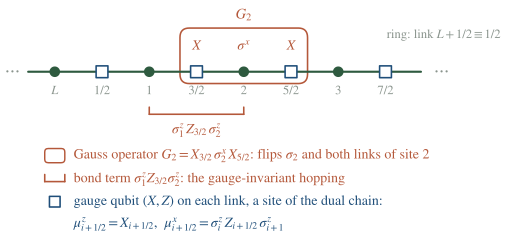
Figure 1. The gauged chain: Ising spins on the sites, gauge qubits on the links, the Gauss operator of site 2, and the variables of the dual chain, which live on the links.

3.2 The partition function is the cocycle sum

The thermal partition function of the gauged chain is $Z_G=\mathrm{Tr}\left(P{e}^{-H_G/T}\right)$, with the Gauss projector

$$P=\prod _i\frac{1}{2}(1+G_i)=2^{-L}\sum _{\lambda \in C^0}\prod _i{G}_i^{{\lambda }_i}=2^{-L}\sum _{\lambda }{V}_{\lambda }\otimes \prod _i{X}_{i+\frac{1}{2}}^{(d\lambda {)}_{i+1/2}},\text{\hspace{1em}(3.3)}$$

where the last form collects the two factors $X$ that $G_i$ and $G_{i+1}$ put on the link $i+\frac{1}{2}$. We evaluate the trace over the links in the $Z$ eigenbasis $|a⟩$. $H_G$ is diagonal in $a$ and acts on the spins as $H[a]$, and $⟨a|{\prod }_i{X}_{i+1/2}^{(d\lambda {)}_{i+1/2}}|a⟩={\delta }_{d\lambda ,0}$, which keeps $\lambda =0$ and $\lambda \equiv 1$, with $V_1=\eta$. Therefore $Z_G=2^{-L}{\sum }_{a\in C^1}\mathrm{Tr}[(1+\eta )e^{-H[a]/T}]$. Since $V_{\lambda }$ commutes with η, the trace depends on $a$ only through $h$, and each value of $h$ is taken by $2^{L-1}$ cochains, so that

$$Z_G=\frac{1}{2}\sum _{h,h^{\prime }\in {\mathbb{Z}}_2}\mathrm{Tr}\left({\eta }^{h^{\prime }}{e}^{-H_h/T}\right)\equiv \frac{1}{2}\sum _{h,h^{\prime }}{Z}_{h,h^{\prime }}.\text{\hspace{1em}(3.4)}$$

This is (2.5) with $p=0$ on the spacetime torus: $(h,h^{\prime })\in H^1(T^2,{\mathbb{Z}}_2)$ are the spatial and temporal holonomies, a temporal holonomy is an insertion of η in the trace, and $\frac{1}{2}=1/|H^0|$. The factor $2^{-L}$ of the projector and the $2^{L-1}$ cochains per class combine into exactly this ratio. We checked (3.4) for $L=3,\dots ,6$ at $g=0.6$, $T=0.7$, to relative accuracy $10^{-9}$.

3.3 Gauge-invariant operators and the dual chain

The operators that commute with every $G_i$ are generated by ${\sigma }_i^x$, $X_{i+1/2}$ and ${\sigma }_i^z{Z}_{i+1/2}{\sigma }_{i+1}^z$; the spin ${\sigma }_i^z$ alone anticommutes with $G_i$. Define on each link

$${\mu }_{i+\frac{1}{2}}^z=X_{i+\frac{1}{2}},{\mu }_{i+\frac{1}{2}}^x={\sigma }_i^z{Z}_{i+\frac{1}{2}}{\sigma }_{i+1}^z.\text{\hspace{1em}(3.5)}$$

They form a Pauli algebra: ${\mu }_{i+1/2}^x$ and ${\mu }_{i+1/2}^z$ anticommute through $Z_{i+1/2}{X}_{i+1/2}$, and operators on different links commute, since the ${\mu }^x$ are products of mutually commuting $Z$-type operators and each ${\mu }^z$ acts only on its own link. On physical states $G_i=1$ gives ${\sigma }_i^x=X_{i-1/2}{X}_{i+1/2}={\mu }_{i-1/2}^z{\mu }_{i+1/2}^z$, and

$$H_G(g){|}_{\mathrm{phys}}=-\sum _i({\mu }_{i+\frac{1}{2}}^x+g{\mu }_{i-\frac{1}{2}}^z{\mu }_{i+\frac{1}{2}}^z),\text{\hspace{1em}(3.6)}$$

which is $gH(1/g)$ written on the dual chain: the transverse field of $T$ has become the bond of the dual chain, and the bond has become the transverse field. The $4^L$ products of the μ’s are linearly independent on the physical space, whose dimension is $2^L$ (§3.4), so the μ’s act irreducibly and (3.6) holds on the whole physical space. We checked $H_{G}P=H_{\mathrm{dual}}(\mu )P$ as an operator identity on the $4^L$-dimensional space for $L=3,\dots ,6$.

3.4 The orbifold Hilbert space

The $L$ Gauss operators are independent, since a product ${\prod }_{i\in S}{G}_i$ over a nonempty set $S$ flips the spins of $S$ and cannot be the identity; the physical space therefore has dimension $4^L/2^L=2^L$. Two global facts fix its content. First, every link appears in two Gauss operators, so

$$\prod _i{G}_i=\eta ,\text{\hspace{1em}(3.7a)}$$

and every physical state has $\eta =1$: gauging projects onto the symmetric states. Second, the Gauss law relates link configurations by $a\to a+d\lambda$, so every orbit contains the representative with $a=h$ on the link $L+\frac{1}{2}$ and $a=0$ elsewhere, and the physical states of holonomy $h$ are the η-even states of $H_h$. Thus

$${\mathcal{H}}_{\mathrm{phys}}\cong {\mathcal{H}}_0^{\mathrm{even}}\oplus {\mathcal{H}}_1^{\mathrm{even}},H_G{|}_{\mathrm{phys}}\cong H_0{|}_{\mathrm{even}}\oplus H_1{|}_{\mathrm{even}},2^L=2^{L-1}+2^{L-1}.\text{\hspace{1em}(3.7b)}$$

This is the orbifold structure: the invariant states of every twisted sector, the untwisted one included. Combined with (3.6) it gives

$$\mathrm{spec}gH(1/g)=\mathrm{spec}{H}_0(g){|}_{\mathrm{even}}\cup \mathrm{spec}{H}_1(g){|}_{\mathrm{even}},\text{\hspace{1em}(3.7c)}$$

which we checked for $L=3,\dots ,6$ at several $g$.

3.5 The quantum dual symmetry and the operators that change status

The holonomy of the new gauge field,

$$\hat{\eta }=\prod _i{Z}_{i+\frac{1}{2}}=\prod _i{\mu }_{i+\frac{1}{2}}^x(\text{on physical states}),\text{\hspace{1em}(3.8)}$$

commutes with $H_G$ and with every $G_i$, which contains two of its anticommuting partners; the second form holds because each ${\sigma }_i^z$ appears twice in the product of the ${\mu }^x$. On the gauge-fixed representatives $\hat{\eta }=(-1{)}^h$, so the two summands of (3.7b) are its eigenspaces:

$$\mathrm{spec}{H}_G{|}_{\hat{\eta }=+1}=\mathrm{spec}{H}_0{|}_{\mathrm{even}},\mathrm{spec}{H}_G{|}_{\hat{\eta }=-1}=\mathrm{spec}{H}_1{|}_{\mathrm{even}},\text{\hspace{1em}(3.9)}$$

checked for $L=3,\dots ,6$. By (3.8), $\hat{\eta }$ is the ${\mathbb{Z}}_2$ symmetry of the dual chain (3.6). In spacetime it is the Wilson line of the new gauge field along the spatial circle at fixed time, an operator of codimension 1 in $d=2$: a ${\mathbb{Z}}_2^{(0)}$ symmetry, as $d-p-2=0$ requires (conventions §6). Applying (3.9) to the dual chain at coupling $1/g$ gives $\mathrm{spec}{H}_0(g){|}_{\mathrm{odd}}=\mathrm{spec}g{H}_1(1/g){|}_{\mathrm{even}}$, also checked: the odd states of the periodic chain are matched by the even states of the antiperiodic chain at the dual coupling, the sector mixing announced in Sem I Week 4 §4.4.

Two kinds of operators change status. (i) The local operator ${\mu }_{i+1/2}^z=X_{i+1/2}$ anticommutes with $\hat{\eta }$: it carries the dual charge. On physical states, for $a<b$, the product of the Gauss laws $G_{a+1}\cdots G_b$ gives

$${\mu }_{a+\frac{1}{2}}^z{\mu }_{b+\frac{1}{2}}^z=X_{a+\frac{1}{2}}{X}_{b+\frac{1}{2}}=\prod _{j=a+1}^b{\sigma }_j^x,\text{\hspace{1em}(3.10)}$$

the segment of the η line between the dual sites $a+\frac{1}{2}$ and $b+\frac{1}{2}$, which is the Kadanoff–Ceva disorder pair of Sem I Week 4 §4.1 in Hamiltonian form. In $T$ the segment is a piece of a topological line whose endpoints cannot be separated from it; in $T/{\mathbb{Z}}_2$ the line has become trivial and each endpoint is a local operator in its own right. (ii) The order parameter loses its status. ${\sigma }_i^z$ anticommutes with $G_i$, and the gauge-invariant completion of the two-point operator is the open Wilson line

$${\sigma }_a^z{Z}_{a+\frac{1}{2}}{Z}_{a+\frac{3}{2}}\cdots Z_{b-\frac{1}{2}}{\sigma }_b^z={\mu }_{a+\frac{1}{2}}^x{\mu }_{a+\frac{3}{2}}^x\cdots {\mu }_{b-\frac{1}{2}}^x,\text{\hspace{1em}(3.11)}$$

a segment of the dual symmetry line (3.8): ${\sigma }_a^z$ is now the endpoint of a topological line of $T/{\mathbb{Z}}_2$, the mirror image of (3.10). We checked the gauge invariance of (3.11) and the anticommutation of ${\sigma }_i^z$ with $G_i$ on the chains with $L=3,\dots ,6$. Figure 2 summarizes the exchange.

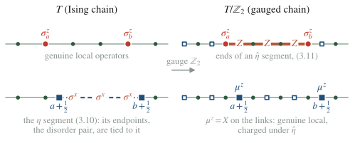
Figure 2. Gauging exchanges order and disorder operators. The endpoints of the η segment, the Kadanoff–Ceva disorder pair, become local operators charged under the dual symmetry η̂, while the order parameter ${\sigma }^z$ becomes the endpoint of a segment of the η̂ line.

Physical picture. What a numerical diagonalization of $T/{\mathbb{Z}}_2$ shows follows from (3.9); the identities are exact, and the large-$L$ statements are the standard behaviour of the two phases of the chain. In the paramagnet of $T$, $g>1$, the twist is invisible at long distances: $H_0$ and $H_1$ have even ground states whose splitting vanishes as $L\to \infty$ (for $L=3$ and $g=2$ they are $-3-2\sqrt{3}$ and $-1-2\sqrt{7}$, already within 3% of each other), and by (3.9) the gauged chain has two nearly degenerate ground states with $\hat{\eta }=\pm 1$: the dual symmetry is spontaneously broken. In the ferromagnet of $T$, $g<1$, the twist costs a domain wall, only the η-even cat state survives the projection, and $T/{\mathbb{Z}}_2$ is a paramagnet. Gauging thus exchanges ordered and disordered phases while keeping every energy level, which is Kramers–Wannier duality read as a statement about phases.

3.6 Kramers–Wannier is gauging

The duality operator of Sem I Week 4 §4.4 is a composite of three maps: couple $T$ to the trivial background, $E|s⟩=|s⟩\otimes |a=0⟩$; project with $P$; and identify the physical space with a chain on the original sites, by reading the dual chain in its ${\mu }^z$ basis and moving each dual site $i+\frac{1}{2}$ to the site $i+1$ (the map $R$). By (3.5) and the Gauss law the dual basis states are product states in the $X$ basis,

$$|m⟩⟩=\underset{i}{⨂}|{\sigma }_i^x=(-1{)}^{m_{i-1/2}+m_{i+1/2}}⟩\otimes \underset{i}{⨂}|X_{i+1/2}=(-1{)}^{m_{i+1/2}}⟩,$$

with $|\pm ⟩=(|0⟩\pm |1⟩)/\sqrt{2}$, so that ${\mu }_{i+1/2}^z|m⟩⟩=(-1{)}^{m_{i+1/2}}|m⟩⟩$ and ${\mu }_{i+1/2}^x$ flips $m_{i+1/2}$ with no phase, since ${\sigma }^z$ and $Z$ exchange $|+⟩$ and $|-⟩$. As $|m⟩⟩$ is physical, $⟨⟨m|PE|s⟩=⟨⟨m|E|s⟩$, and each site contributes $⟨\pm |s_i⟩=2^{-1/2}(-1{)}^{s_i(m_{i-1/2}+m_{i+1/2})}$ and each link $⟨\pm |0⟩=2^{-1/2}$:

$$⟨⟨m|PE|s⟩=2^{-L}(-1{)}^{{\sum }_i{s}_i(m_{i-1/2}+m_{i+1/2})}.$$

With the relabeling $m_{i+1/2}=s_{i+1}^{\prime }$ and the factor $2^{L/2}$ that makes $D^{†}D=1+\eta$ exact (below), the composite is

$$\boxed{D=2^{L/2}RPE=2^{-L/2}\sum _{s,s^{\prime }}(-1{)}^{\Phi (s,s^{\prime })}|s^{\prime }⟩⟨s|,\Phi (s,s^{\prime })=\sum _i{s}_i(s_i^{\prime }+s_{i+1}^{\prime }),}\text{\hspace{1em}(3.12)}$$

real in the ${\sigma }^z$ basis, as Sem I Week 4 §4.4 and conventions §4 require.

The relations of conventions §4 follow from the bilinear phase Φ in one line each. Flipping $s_i$ changes Φ by $s_i^{\prime }+s_{i+1}^{\prime }$, so $D{\sigma }_i^x={\sigma }_i^z{\sigma }_{i+1}^{z}D$; flipping $s_{i+1}^{\prime }$ changes it by $s_i+s_{i+1}$, so $D{\sigma }_i^z{\sigma }_{i+1}^z={\sigma }_{i+1}^{x}D$. For the products, with $u=s+t$ and $\Phi (s,s^{\prime })+\Phi (t,s^{\prime })={\sum }_i{s}_i^{\prime }(u_i+u_{i-1})$,

$$(D^{†}D{)}_{ts}=2^{-L}\sum _{s^{\prime }}(-1{)}^{{\sum }_i{s}_i^{\prime }(u_i+u_{i-1})}={\delta }_{u,0}+{\delta }_{u,1},\text{so}{D}^{†}D=1+\eta ,$$

and in the same way $(D^2{)}_{s^{\prime \prime }s}=1$ exactly when $s_i^{\prime \prime }+s_{i+1}^{\prime \prime }=s_{i-1}+s_i$ for every $i$, and 0 otherwise. The two solutions $s_i^{\prime \prime }=s_{i-1}$ and $s_i^{\prime \prime }=s_{i-1}+1$ give $D^2=(1+\eta )T$ with $(Ts{)}_i=s_{i-1}$, which is $T{\sigma }_i{T}^{-1}={\sigma }_{i+1}$. Finally $D_{Tx,s}=2^{-L/2}(-1{)}^{{\sum }_i{s}_i(x_{i-1}+x_i)}=2^{-L/2}(-1{)}^{\Phi (x,s)}=(D^{†}{)}_{x,s}$, so $D^{†}=T^{-1}D$, and the same reindexing gives $DT=TD$. The intertwining $DH(g)=gH(1/g)D$ follows from $EH(g)=H_G(g)E$ (the background is trivial), $[P,H_G]=0$ and (3.6). We compared (3.12) with the composite $2^{L/2}RPE$ built numerically on the $4^L$-dimensional gauged chain, and checked every relation of this paragraph, for $L=3,\dots ,6$.

The construction explains why $D$ cannot be inverted. $P$ annihilates the η-odd states by (3.7a), so $D\eta =\eta D=D$; and $E$ creates the trivial holonomy, which $P$ preserves, so the image of $D$ lies in the $\hat{\eta }=+1$ sector. The twisted sector of $T/{\mathbb{Z}}_2$, which by §3.5 carries the odd states of $T$ at the dual coupling, is never reached from the periodic chain. The half-site shift $i+\frac{1}{2}\mapsto i+1$ is a choice: moving the dual sites to $i$ instead gives $T^{-1}D$, and the choice of conventions §4 is the one that puts $T$ in $D^2$. Building $D$ as a topological line in spacetime requires gauging in half of spacetime, which is Sem II Week 13.

3.7 The three-site chain in full [Computed.]

For $L=3$ we order the basis as $|s_1{s}_2{s}_3⟩$ with index $4s_1+2s_2+s_3$. Then

$$H_0(g)=\mathrm{diag}(-3,1,1,1,1,1,1,-3)-g{A}_3,H_1(g)=\mathrm{diag}(-1,-1,3,-1,-1,3,-1,-1)-g{A}_3,$$

where $(A_3{)}_{s^{\prime }s}=1$ when $s$ and $s^{\prime }$ differ in exactly one spin (the adjacency matrix of the cube) and the antiperiodic bond is the one between sites 3 and 1. The symmetry is $\eta |s⟩=|s+111⟩$, the translation is $T|s_1{s}_2{s}_3⟩=|s_3{s}_1{s}_2⟩$, and (3.12) is

$$2^{3/2}D=\left(\begin{array}{cccccccc}1& 1& 1& 1& 1& 1& 1& 1\\ 1& -1& -1& 1& 1& -1& -1& 1\\ 1& 1& -1& -1& -1& -1& 1& 1\\ 1& -1& 1& -1& -1& 1& -1& 1\\ 1& -1& 1& -1& -1& 1& -1& 1\\ 1& 1& -1& -1& -1& -1& 1& 1\\ 1& -1& -1& 1& 1& -1& -1& 1\\ 1& 1& 1& 1& 1& 1& 1& 1\end{array}\right).$$

Row $s^{\prime }$ and row $s^{\prime }+111$ coincide ($\eta D=D$), column $s$ and column $s+111$ coincide ($D\eta =D$), and $D$ has rank 4. In $(2^{3/2}D{)}^{\mathsf{T}}(2^{3/2}D)=8(1+\eta )$ the entries on the diagonal and the antidiagonal equal 8, and every other entry vanishes because two columns that are neither equal nor complementary are orthogonal.

Diagonalizing the $4\times 4$ blocks of definite η gives Table 1, whose closed forms we checked at $g=0.3,0.5,0.8,1.7,2.5$.

sector	eigenvalues	at $g=\frac{1}{2}$
$H_0$, $\eta =+1$	$-(1+g)\mp 2\sqrt{1-g+g^2}$; $1+g$ (twice)	$-3.232051,0.232051,1.5,1.5$
$H_0$, $\eta =-1$	$-(1-g)\mp 2\sqrt{1+g+g^2}$; $1-g$ (twice)	$-3.145751,2.145751,0.5,0.5$
$H_1$, $\eta =+1$	$(1-g)\mp 2\sqrt{1+g+g^2}$; $-(1-g)$ (twice)	$-2.145751,3.145751,-0.5,-0.5$
$H_1$, $\eta =-1$	$(1+g)\mp 2\sqrt{1-g+g^2}$; $-(1+g)$ (twice)	$-0.232051,3.232051,-1.5,-1.5$

Table 1. The four sectors of the three-site chain. By (3.9) the gauged chain has the spectrum of rows 1 and 3, which is the spectrum of $\frac{1}{2}H(2)$, and $g$ times row 3 at $1/g$ is row 2, the sector mixing of §3.5.

4. The degree rule, derived by counting backgrounds [Proved.]

4.1 The dual background

After gauging, $B$ is summed over, and the gauged theory is probed by weighting the sum with a phase that depends on $B$. A gauge-invariant phase linear in $B$ pairs $[B]$ with a class of complementary degree. Let $C\in C^{q^{\prime }}(X,{\mathbb{Z}}_N)$ and define

$$Z_{T/{\mathbb{Z}}_N^{(p)}}[C]={\mathcal{N}}_p\sum _{B\in Z^{p+1}}{Z}_T[B]{\omega }^{{\sum }_{X}B\cup C},\omega =e^{2\pi i/N},\text{\hspace{1em}(4.1)}$$

with the cup product of conventions §8. The sum over $X$ runs over the cells of top degree, so $q^{\prime }=d-p-1$. Under $B\to B+d\lambda$ the Leibniz rule $d(\lambda \cup C)=d\lambda \cup C+(-1{)}^p\lambda \cup dC$ and ${\sum }_{X}d(\cdot )=0$ on closed $X$ give ${\sum }_{X}d\lambda \cup C=-(-1{)}^p{\sum }_X\lambda \cup dC$, so (4.1) is well defined for every λ exactly when $dC=0$. Under $C\to C+d\mu$, $d(B\cup \mu )=(-1{)}^{p+1}B\cup d\mu$ because $dB=0$, and the weight is unchanged. Therefore $C$ is a background gauge field, closed and defined up to exact terms, of degree $d-p-1$, and a background of degree $d-p-1$ couples to a symmetry of degree $d-p-2$:

$$\boxed{{\mathbb{Z}}_N^{(p)}\stackrel{\text{gauging}}{\to }{\hat{\mathbb{Z}}}_N^{(d-p-2)}\cong {\mathbb{Z}}_N^{(d-p-2)},}\text{\hspace{1em}(4.2)}$$

the rule of conventions §6 (written there with $q$ for the degree).

4.2 Counting, and the inverse

The degree is forced by (4.1). The counting shows that nothing is lost. First, $|H^{p+1}(T^d,{\mathbb{Z}}_N)|=N^{\left(\genfrac{}{}{0ex}{}{d}{p+1}\right)}=N^{\left(\genfrac{}{}{0ex}{}{d}{d-p-1}\right)}=|H^{d-p-1}(T^d,{\mathbb{Z}}_N)|$: the gauged theory has exactly as many dual backgrounds as $T$ had backgrounds. Second, the pairing $⟨[B],[C]⟩={\sum }_{X}B\cup C$ is perfect (Poincaré duality, Sem I Week 2). On $T^d$ the classes are represented by the seams $e^S=e^{{\mu }_1}\cup \cdots \cup e^{{\mu }_k}$, $S=\{{\mu }_1<\cdots <{\mu }_k\}$, where $e^{\mu }$ equals 1 on the μ-links with $x_{\mu }=0$; the cup formula of conventions §8 gives $e^S(x;S)=1$ exactly when $x_{\mu }=0$ for $\mu \in S$, and ${\sum }_X{e}^S\cup e^{S^{\prime }}=ϵ(S,S^{\prime })$ if $S^{\prime }$ is the complement of $S$ and 0 otherwise, with the shuffle sign of §8. We checked that the resulting pairing matrices are unimodular on $T^3$ and $T^4$ ($L=2$, $N=2,3$). Third, gauging the dual symmetry with the opposite sign of the coupling inverts the operation:

$${\mathcal{N}}_{d-p-2}\sum _{C\in Z^{d-p-1}}{Z}_{T/{\mathbb{Z}}_N^{(p)}}[C]{\omega }^{-{\sum }_X{B}^{\prime }\cup C}={\mathcal{N}}_{d-p-2}{\mathcal{N}}_p\sum _B{Z}_T[B]\sum _C{\omega }^{{\sum }_X(B-B^{\prime })\cup C}.\text{\hspace{1em}(4.3)}$$

By perfectness and the orthogonality of characters the $C$-sum is $|B^{d-p-1}||H^{d-p-1}|{\delta }_{[B],[B^{\prime }]}$, and the $B$-sum then gives $|B^{p+1}|Z_T[B^{\prime }]$. By (2.5) the constant is the product of the two ratios of (2.5), for degrees $p$ and $d-p-2$, times $|H^{d-p-1}|$, and Poincaré duality $|H^k|=|H^{d-k}|$ reduces it to ${\prod }_k|H^k{|}^{\pm (-1{)}^k}=N^{\pm \chi (X)}$. On the torus $\chi =0$, so

$$(T/{\mathbb{Z}}_N^{(p)})/{\hat{\mathbb{Z}}}_N^{(d-p-2)}=T\text{on }{T}^d,\text{with its background }{B}^{\prime }.\text{\hspace{1em}(4.4)}$$

With the same sign in both couplings, (4.3) returns $Z_T[-B^{\prime }]$, the charge-conjugate theory (F7). We checked that the product of normalizations is 1 for every $(d,p)$ with $d-p-2\ge 0$ on the tori of §2.2, and we checked (4.3) for the chiral ${\mathbb{Z}}_3$ clock model, $w(n)=e^{K\cos (2\pi n/3+\psi )}$ at $K=0.45$, $\psi =0.3$, on the $2\times 3$ torus, where $Z[a]\ne Z[-a]$: (4.3) returns $Z_T[B^{\prime }]$, and the other sign returns $Z_T[-B^{\prime }]$.

The rule in the dimensions of the course, with the Semester I examples:

$d$	$p=0$	$p=1$	$p=2$
2	$0$: Kramers–Wannier (§§3, 4.4)	$-1$ (F6)
3	$1$: Ising $\to$ ${\mathbb{Z}}_2$ gauge theory (Sem I Week 5 §7; §4.4)	$0$: ${\mathbb{Z}}_2$ gauge theory $\to$ Ising (Mini-calculation 1)	$-1$
4	$2$: vortex sheets become genuine	$1$: self-duality of 4d ${\mathbb{Z}}_2$ gauge theory (Sem I Week 5 §8.3); $SU(N)\to SU(N)/{\mathbb{Z}}_N$ (§6)	$0$

4.3 What becomes genuine [Proved for the models (2.1).]

Four statements, each proved by a change of the summation variable in (4.1).

(a) The generators of the dual symmetry are the Wilson operators of $B$, $V_j(\Sigma )={\omega }^{j{\sum }_{\Sigma }B}$ on closed $(p+1)$-cycles Σ, of codimension $d-p-1=(d-p-2)+1$ as a $(d-p-2)$-form symmetry requires. They are topological: for homologous cycles ${\Sigma }^{\prime }-\Sigma =\partial V$, and ${\sum }_{\partial V}B={\sum }_{V}dB=0$.

(b) A symmetry operator $U_s(M)$ of $T$ on a closed $(d-p-1)$-cycle $M$ shifts $B$ by $s{\delta }_M$, with ${\delta }_M$ the closed $(p+1)$-cochain Poincaré dual to $M$ (the transport rule of conventions §2). In $T/{\mathbb{Z}}_N$ the relabeling $B\to B-s{\delta }_M$ removes it, at the cost of the c-number ${\omega }^{-s{\sum }_X{\delta }_M\cup C}$: the gauged symmetry operators are trivial, up to a phase set by the dual background.

(c) An open $U_s(M)$ with $\partial M=\gamma$, of dimension $d-p-2$, is a twisted-sector operator of $T$, tied to $M$. In $T/{\mathbb{Z}}_N$ two choices of $M$ with the same boundary differ by a closed cycle, which (b) removes, so the operator depends only on γ: it is genuine, and its dimension is the degree of the dual symmetry, under which it carries charge $s$ through the linking with $V_j$. The disorder operators of (3.10) are the case $d=2$, $p=0$.

(d) A charged operator $O_e$ of $T$, of charge $e$ and supported on a $p$-cycle, changes under $\varphi \to \varphi +\lambda$, while $O_e{\omega }^{-e{\sum }_{\Gamma }B}$ with $\partial \Gamma =\mathrm{supp}{O}_e$ is invariant: $O_e$ becomes the boundary of a dual-symmetry operator, as ${\sigma }^z$ did in (3.11).

GKSW state (a)–(d) on pp. 11–12 [Stated there; the change of variables proves them for the models (2.1)], with the remark that gauging the dual symmetry gives back the original theory, which is (4.4).

4.4 Kramers–Wannier on the torus is gauging [Computed.]

For the 2d Ising model at coupling $K$ (written β in Sem I Week 4 §3) the sector partition functions $Z_{ϵ}(K)$ of Sem I Week 4 §3.4 are $Z[a_{ϵ}]$ for a seam background with holonomies $ϵ$: $a_{ϵ,1}$ equals ${ϵ}_1$ on the 1-links with $x_1=0$, and $a_{ϵ,2}$ equals ${ϵ}_2$ on the 2-links with $x_2=0$. The two-term cup product of conventions §8 gives

$$\sum _P{a}_{ϵ}\cup a_c=\sum _x[a_{ϵ,1}(x)a_{c,2}(x+\hat{1})-a_{ϵ,2}(x)a_{c,1}(x+\hat{2})]={ϵ}_1{c}_2-{ϵ}_2{c}_1,$$

since each term is nonzero only at $x=(0,0)$. Mod 2 this is the crosswise pairing of the boxed formula of Sem I Week 4 §3.4, so that formula, multiplied by ${\sinh }^{N_s}2K$, is (4.1) for $p=0$, $d=2$:

$$Z_{T/{\mathbb{Z}}_2}[c](K)={\sinh }^{N_s}(2K)Z_c(K^{\ast }),\sinh 2K\sinh 2K^{\ast }=1,\text{\hspace{1em}(4.5)}$$

on every $L_1\times L_2$ torus with $N_s$ sites: the Ising model at $K$, gauged and coupled to the dual background $c$, is the Ising model at $K^{\ast }$ coupled to $c$, up to an analytic factor. At $K_c=\frac{1}{2}\ln (1+\sqrt{2})$ the vector of the four $Z_{ϵ}$ is invariant under the gauging matrix $M_{cϵ}=\frac{1}{2}(-1{)}^{{ϵ}_1{c}_2+{ϵ}_2{c}_1}$, which squares to 1 by (4.4): self-duality is invariance under gauging. We rechecked (4.5) by enumeration on the $2\times 3$, $3\times 3$, $3\times 4$ and $2\times 5$ tori; the dot pairing fails on the three non-square ones.

In $d=3$ the torus form of Wegner’s duality (conventions §4) is $2^{N_{\ell }}(2\sinh 2K^{\ast }{)}^{-N_P/2}$ times $\frac{1}{2}{\sum }_{ϵ\in H^1(T^3,{\mathbb{Z}}_2)}{Z}_I^{(ϵ)}(K^{\ast })$, the normalized sum (2.5) for $p=0$: Wegner’s gauge theory at β is the Ising model at $K^{\ast }$ with its ${\mathbb{Z}}_2^{(0)}$ gauged, normalization included [Stated — refs: Sem I Week 5 §7.1 and F6]. Its dual ${\mathbb{Z}}_2^{(1)}$ is Wegner’s electric 1-form symmetry: the Ising spin, tied by §4.3(d) to a dual-symmetry line, is the vison at the end of an open flipped sheet (Sem I Week 5 §7.3), and the boundaries of open Ising domain walls, made genuine by §4.3(c), are Wegner’s Wilson loops (Sem I Week 5 §7.2). Mini-calculation 1 gauges in the opposite direction.

5. Gauging a subgroup

5.1 The exact sequence, gauged [Proved.]

Let $H=⟨k⟩\subset {\mathbb{Z}}_N$, $r=\gcd (N,k)$ and $N^{\prime }=N/r$, so that $H=r{\mathbb{Z}}_N\cong {\mathbb{Z}}_{N^{\prime }}$, the notation of Sem I Week 14 §3 with $q\to k$. Gauging $H$ means summing over $B\in Z^{p+1}(X,H)$ in (2.4), with $\lambda \in C^p(X,H)$ and the normalization computed with $H$ in place of ${\mathbb{Z}}_N$. Charges $e$ and symmetry elements $s$ are paired by ${\omega }^{se}$. The arguments of §4.3 with λ restricted to $H$ give four statements.

(i) Genuine charged operators. $O_e$ is invariant under $\lambda \in C^p(X,H)$ exactly when ${\omega }^{eh}=1$ for all $h\in H$, that is $e\in \mathrm{Ann}(H)=N^{\prime }{\mathbb{Z}}_N\cong {\mathbb{Z}}_r$. For other $e$ the invariant object is $O_e{\omega }^{-e{\sum }_{\Gamma }B}$, and since $B$ is $H$-valued this phase depends on $e$ only through ${\mathrm{res}}_H(e)\in \hat{H}$. The sequence (3.5) of Sem I Week 14,

$$0⟶\mathrm{Ann}(H)⟶{\mathbb{Z}}_N\stackrel{{\mathrm{res}}_H}{\to }\hat{H}⟶0,\text{\hspace{1em}(5.1)}$$

now reads as follows: the kernel is the set of charges that stay genuine, and the image says to which operator of the dual symmetry $\hat{H}$ every other charge is tied.

(ii) Residual symmetry. The shifts by ${\mathbb{Z}}_N$ modulo the gauged ones form ${\mathbb{Z}}_N/H\cong {\mathbb{Z}}_r$, of degree $p$, acting on the genuine operators; the pairing descends to a perfect pairing of $\mathrm{Ann}(H)$ with ${\mathbb{Z}}_N/H$ (Sem I Week 14 §3.3).

(iii) Dual symmetry. $\hat{H}\cong {\mathbb{Z}}_{N^{\prime }}$, of degree $d-p-2$, generated by $V_j(\Sigma )=e^{2\pi ij{\sum }_{\Sigma }b/N^{\prime }}$ with $B=rb$, $b\in {\mathbb{Z}}_{N^{\prime }}$.

(iv) Newly genuine operators. The boundaries of $U_s(M)$ with $s\in H$, by §4.3(c). For $s\notin H$ the open operator remains tied to the residual-symmetry operator $U_{[s]}(M)$.

	$N=6$, $k=4$	$N=4$, $k=2$
$r$, $N^{\prime }$	2, 3	2, 2
gauged $H$	$\{0,2,4\}\cong {\mathbb{Z}}_3$	$\{0,2\}\cong {\mathbb{Z}}_2$
genuine charges $\mathrm{Ann}(H)$	$\{0,3\}\cong {\mathbb{Z}}_2$	$\{0,2\}\cong {\mathbb{Z}}_2$
residual ${\mathbb{Z}}_N/H$, degree $p$	${\mathbb{Z}}_2$	${\mathbb{Z}}_2$
dual $\hat{H}$, degree $d-p-2$	${\mathbb{Z}}_3$	${\mathbb{Z}}_2$
$0\to H\to {\mathbb{Z}}_N\to {\mathbb{Z}}_N/H\to 0$	splits: ${\mathbb{Z}}_6\cong {\mathbb{Z}}_3\times {\mathbb{Z}}_2$	does not split

The last row has physical content. When the extension splits, ${\mathbb{Z}}_N\cong H\times {\mathbb{Z}}_N/H$ and the gauged theory has the product symmetry ${\mathbb{Z}}_r^{(p)}\times {\hat{H}}^{(d-p-2)}$ with no relation between the factors. When it does not, the residual and dual symmetries have a mixed ‘t Hooft anomaly fixed by the extension class [Stated — refs: Tachikawa, arXiv:1712.09542, the first of the three cases of its abstract, for $p=0$ and a non-anomalous parent symmetry]. The extension splits exactly when $\gcd (r,N^{\prime })=1$, which we checked by enumerating all subgroups for $2\le N\le 12$ (Problem 3).

5.2 The ${\mathbb{Z}}_4$ chain: a fractional residual charge [Computed.]

On each site of a ring put the ${\mathbb{Z}}_4$ clock $Z_i$ and shift $X_i$ of conventions §6, with $ZX=\omega XZ$ and $\omega =i$, and take $H_4(g)=-{\sum }_i(Z_i^{†}{Z}_{i+1}+h.c.)-g{\sum }_i(X_i+X_i^{†})$, with the symmetry $U={\prod }_i{X}_i$ generating ${\mathbb{Z}}_4^{(0)}$. Gauge $H=\{0,2\}$, generated by $U^2$: a ${\mathbb{Z}}_2$ qubit on each link, the coupling $Z_i^{†}{Z}_{i+1}\to Z_i^{†}{Z}_{i+1/2}{Z}_{i+1}$, and Gauss operators $G_i=X_{i-1/2}{X}_i^2{X}_{i+1/2}$. Since $X_i^2{Z}_i{X}_i^{-2}=-Z_i$, each bond term at site $i$ picks two signs under $G_i$, and $G_i$ commutes with the gauged Hamiltonian; so does $U$, which also commutes with every $G_i$. Every link appears in two Gauss operators, so

$$U^2=\prod _i{X}_i^2=\prod _i{G}_i.\text{\hspace{1em}(5.2)}$$

On physical states $U^2=1$, and $U$ generates the residual ${\mathbb{Z}}_4/H\cong {\mathbb{Z}}_2$. The twisted sector of the dual symmetry, the Hilbert space with a Wilson line of the $H$ gauge field running in time at the site $i_0$, is the space with $G_{i_0}=-1$ and $G_i=1$ elsewhere, a static $H$-charge. There $U^2=-1$: the residual ${\mathbb{Z}}_2$ acts with eigenvalues $\pm i$. The only lifts of the residual generator are $U$ and $U^3$, and $(U^3{)}^2=U^6=U^2$, so no lift squares to 1 in this sector. For $N=6$ and $H=\{0,2,4\}$ the lift $U^3$ of the residual ${\mathbb{Z}}_2$ satisfies $(U^3{)}^2=U^6=1$ identically, and nothing fractionalizes, in accordance with the splitting of ${\mathbb{Z}}_6$. The fractional residual charge in the dual-twisted sector is the Hilbert-space face of the mixed anomaly of §5.1, the subject of Sem II Week 5. We checked (5.2), the commutators, and $U^2=\pm 1$ on the two sectors for $L=3$, where the physical space has dimension $4^3=64$. Sem I Week 14 F1 compares gauging with screening by charge-$k$ matter, and Sem II Week 14 gauges $H=⟨k⟩$ on a hypersurface, where (5.1) organizes the charge filter of the wall that the group’s manuscript in preparation studies [Stated — forward reference to Sem II Week 14, condensation-defects and the master-project].

6. Global forms: $SU(N)$ and $SU(N)/{\mathbb{Z}}_N$

6.1 The ${\mathbb{Z}}_N$ toy on the lattice [Proved.]

Take ${\mathbb{Z}}_N$ lattice gauge theory in $d=4$, $S=-\beta {\sum }_P\cos (2\pi (da{)}_P/N)$, the model of conventions §4 without matter. Its Wilson loops $W_e(C)={\omega }^{e{\sum }_{C}a}$ are genuine for every $e\in {\mathbb{Z}}_N$. Its ‘t Hooft loop $T_m(\tilde{C})$ replaces $(da{)}_P$ by $(da{)}_P-m$ on the plaquettes dual to a dual surface $\tilde{S}$ with $\partial \tilde{S}=\tilde{C}$ (conventions §6), and moving $\tilde{S}$ across a Wilson loop $W_e$ multiplies the correlator by ${\omega }^{\pm em}$, the linking action of Sem II Week 1 §5. Since $e=1$ is present, $T_m$ with $m\ne 0$ stays tied to its surface, which is the electric symmetry operator $U_m$. In the language of AST §1.1, the genuine line classes $(z_e,z_m)$ of the toy are ${\mathbb{Z}}_N\times \{0\}$, the line content of $SU(N)$.

Write $N=k{k}^{\prime }$ and gauge the subgroup $H=k^{\prime }{\mathbb{Z}}_N$ of order $k$ of the electric ${\mathbb{Z}}_N^{(1)}$ (in the notation of §5, $H=⟨k^{\prime }⟩$, $r=k^{\prime }$, $N^{\prime }=k$):

$$Z={\mathcal{N}}_1\sum _{B\in C^2(\Lambda ,H),dB=0}\sum _a\prod _P{e}^{\beta \cos (2\pi (da-B{)}_P/N)},a\to a+\lambda ,B\to B+d\lambda ,\lambda \in C^1(\Lambda ,H).\text{\hspace{1em}(6.1)}$$

The ‘t Hooft loop of charge $m\in H$ is the insertion that replaces the constraint by $dB=m{J}_{\tilde{C}}$, where $J_{\tilde{C}}$ is the 3-cochain Poincaré dual to $\tilde{C}$. Its solutions are $B_0+m{\delta }_{\tilde{S}}$ with $B_0$ closed and $\tilde{S}$ any dual surface bounded by $\tilde{C}$, so this is the twist of conventions §6 on $\tilde{S}$, now manifestly independent of $\tilde{S}$. Three statements follow.

(i) $W_e$ is invariant under $\lambda \in C^1(\Lambda ,H)$ exactly when $e\in \mathrm{Ann}(H)=k{\mathbb{Z}}_N$; for other $e$ it is tied to ${\omega }^{-e{\sum }_{\Gamma }B}$ with $\partial \Gamma =C$, by §5.1(i).

(ii) $T_m$ is genuine for $m\in H=k^{\prime }{\mathbb{Z}}_N$. For $m\notin H$ the equation $dB=m{J}_{\tilde{C}}$ has no $H$-valued solution, the twist on $\tilde{S}$ cannot be absorbed, and the surface is the residual-symmetry operator $U_m$, which acts on the genuine $W_k$ by ${\omega }^{km\mathrm{Link}}\ne 1$.

(iii) The dual symmetry ${\hat{H}}^{(1)}\cong {\mathbb{Z}}_k^{(1)}$, of degree $4-1-2=1$, is generated by $V_j(\Sigma )=e^{2\pi ij{\sum }_{\Sigma }b/k}$ with $B=k^{\prime }b$, and for $\Sigma =\partial V$ and $m=k^{\prime }{m}^{\prime }$, Stokes gives ${\sum }_{\partial V}B={\sum }_{V}dB=m\#(V\cap \tilde{C})$, so

$$V_j(\partial V)\text{in the presence of}{T}_m(\tilde{C})=e^{2\pi ij{m}^{\prime }\#(V\cap \tilde{C})/k},\text{\hspace{1em}(6.2)}$$

the linking action, with $\#(V\cap \tilde{C})$ the signed count of the cubes of $V$ dual to the links of $\tilde{C}$, defined as in conventions §6.

The genuine lines of the gauged toy are therefore

$$\{W_e{T}_m:e\in k{\mathbb{Z}}_N,m\in k^{\prime }{\mathbb{Z}}_N\}⟷L_{k,0}=k{\mathbb{Z}}_N\times k^{\prime }{\mathbb{Z}}_N,\text{\hspace{1em}(6.3)}$$

mutually local because $em\in k{k}^{\prime }\mathbb{Z}=N\mathbb{Z}$. The dictionary with $SU(N)$ is a formal analogy for the dynamics and an exact match for the bookkeeping [Formal analogy.]: $W_e$ are the Wilson lines of $N$-ality $e$, $T_m$ the ‘t Hooft lines of magnetic class $m$, the electric ${\mathbb{Z}}_N^{(1)}$ the center symmetry of Sem I Week 14 §4, gauging $H$ the passage from $SU(N)$ to $SU(N)/{\mathbb{Z}}_k$, and ${\hat{H}}^{(1)}$ the magnetic 1-form symmetry of $SU(N)/{\mathbb{Z}}_k$, generated by $\exp (2\pi i\int w_2/k)$ (AST §6.4). The toy reproduces AST’s $L_{k,0}$; the sets $L_{k,n}$ with $n\ne 0$ need a counterterm in the sum over $B$ (§6.2).

6.2 The continuum statement [Stated — refs: AST §§1.1–1.2, 2.1, 2.3, 6.1.]

AST label line operators by classes $(z_e,z_m)\in {\mathbb{Z}}_N\times {\mathbb{Z}}_N$ (their (1.3)) and require mutual locality,

$$z_e{z}_m^{\prime }-z_m{z}_e^{\prime }\equiv 0(\mathrm{mod}N),\text{\hspace{1em}(6.4)}$$

(their (1.4)), together with completeness: the set of genuine lines is maximal. For $\mathfrak{su}(2)$ there are three maximal sets: $SU(2)$, with $(1,0)$; $SO(3{)}_{+}$, with $(0,1)$; and $SO(3{)}_{-}$, with $(1,1)$. Under $\theta \to \theta +2\pi$ the Witten effect sends $(z_e,z_m)\to (z_e+z_m,z_m)$ (their (2.4)), the direction of conventions §10, so that $SO(3{)}_{+}$ at θ is $SO(3{)}_{-}$ at $\theta +2\pi$ (their (1.5)). For general $N$ the maximal sets are

$$L_{k,n}=\{e(k,0)+m(n,k^{\prime })\mathrm{mod}N\},k{k}^{\prime }=N,n=0,\dots ,k-1,\text{\hspace{1em}(6.5)}$$

the line content of $(SU(N)/{\mathbb{Z}}_k{)}_n$ (their (2.8); $L_n=L_{N,n}=\{(nm,m)\}$ is their (2.1)), and $\theta \to \theta +2\pi$ maps $L_{k,n}\to L_{k,n+k^{\prime }}$ (their (2.9)). When $\gcd (k,k^{\prime })>1$, which is possible for some divisor $k$ exactly when $N$ is not square-free, some $n$ are not related by shifts of θ: they are distinguished by a discrete θ-angle, the phase $i\frac{2\pi n}{k}\frac{\mathcal{P}(w_2)}{2}$ in the sum over bundles (their (6.8)), whose lattice form needs the Pontryagin square of Sem II Week 6 (Problem 8⋆⋆).

The combinatorial part of this statement has a short proof [Proved.]. A mutually local set $L$ is a subgroup isotropic for the alternating pairing (6.4). If $x\in L^{\perp }\setminus L$, then $L+⟨x⟩$ is again isotropic, so a maximal $L$ equals $L^{\perp }$ and has $N$ elements, since $|L||L^{\perp }|=N^2$. Its electric part $L\cap ({\mathbb{Z}}_N\times 0)$ is a subgroup $k{\mathbb{Z}}_N\times 0$ for some divisor $k$, of order $k^{\prime }$; the magnetic projection then has order $N/k^{\prime }=k$, so it is $k^{\prime }{\mathbb{Z}}_N$, and $L$ contains some $(n,k^{\prime })$ with $n$ defined modulo $k$. The two generators span $N$ elements, so $L=L_{k,n}$. The number of maximal sets is $\sigma (N)={\sum }_{k|N}k$, which is 7 for $N=4$, 12 for $N=6$ and 28 for $N=12$. We enumerated the isotropic subgroups of order $N$ of ${\mathbb{Z}}_N^2$ for $2\le N\le 12$ and found exactly the sets (6.5), on which $(z_e,z_m)\to (z_e+z_m,z_m)$ acts as stated; the toy sets (6.3) coincide with $L_{k,0}$. Figure 3 shows four of the seven sets for $N=4$.

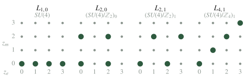
Figure 3. Four of the seven maximal sets of mutually local line classes for N = 4 (large dots = genuine). The ${\mathbb{Z}}_N$ toy of §6.1 without counterterm produces L₁,₀, L₂,₀ and L₄,₀; the shift θ → θ + 2π moves L₄,ₙ to L₄,ₙ₊₁ and fixes both L₂,₀ and L₂,₁, which therefore differ by a discrete θ-angle.

7. Mini-calculation 1 (hand-in)

7.1 Scope

The calculation has two layers. The chain layer is exact on every finite ring and uses only §3. The layer one dimension up is exact on finite spatial tori and uses the Kogut–Susskind ${\mathbb{Z}}_2$ Hamiltonian of conventions §4, $H=-\Gamma {\sum }_{\ell }{\sigma }_{\ell }^x-K{\sum }_P{B}_P$ with $B_P={\prod }_{\ell \in \partial P}{\sigma }_{\ell }^z$ and Gauss law ${\prod }_{\ell \ni v}{\sigma }_{\ell }^x=1$; the electric symmetry operators $U_1$, $U_2$ are those of Sem I Week 15 §3.4. Nothing is claimed about continuum limits or critical exponents. The value $(K/\Gamma {)}_c\approx 3.044$ (Blöte–Deng, in the paper map) is imported only to name the phase of the numerical point of Sub-task 4.

7.2 Variable dictionary

symbol	chain (§3)	one dimension up
${\sigma }^{x,z}$	Ising spins on sites	gauge field on links
$X,Z$	gauge qubits on links	2-form gauge qubits on plaquettes
${\mu }^{x,z}$	dual chain, on links	dual Ising spins, on plaquettes
Gauss law	$G_i=X_{i-1/2}{\sigma }_i^x{X}_{i+1/2}$	$G_{\ell }={\sigma }_{\ell }^x{\prod }_{P\ni \ell }{X}_P$
gauged symmetry	$\eta$, ${\mathbb{Z}}_2^{(0)}$	$U_1,U_2$, ${\mathbb{Z}}_2^{(1)}$
dual symmetry	$\hat{\eta }=\prod Z_{i+1/2}$, ${\mathbb{Z}}_2^{(0)}$	${\prod }_P{Z}_P$, ${\mathbb{Z}}_2^{(0)}$

7.3 Sub-tasks

Sub-task 1: the four-site chain. Build the 8-qubit gauged chain (3.2) for $L=4$, its projector $P$, and the composite $2^{2}RPE$ of §3.6. Display $4D$ as a $16\times 16$ sign matrix, verify the relations of §3.6 and the identities (3.7c) and (3.9) at $g=\frac{1}{2}$. Deliverable: the matrix, the four sector spectra, and the list of checks with their numerical residuals. Checkpoint: $D$ has rank 8; at $g=\frac{1}{2}$ the lowest levels are $-4.271558$ ($H_0$, even), $-4.236068=-(2+\sqrt{5})$ ($H_0$, odd), $-3.236068=-(1+\sqrt{5})$ ($H_1$, even) and $-2.797933$, twofold ($H_1$, odd); the gauged spectrum is the union of the two even sectors and equals that of $\frac{1}{2}H(2)$.

Sub-task 2: the cocycle sum on the torus. Enumerate $C^1$ of the $2\times 3$ torus ($L_1=2$, $L_2=3$, 12 links, with ${ϵ}_1$ the holonomy along the length-2 direction), select the closed cochains, and verify $|Z^1|=128$, the class-function property and (2.5). At $K_c$ compute the four $Z_{ϵ}$ and verify that they are invariant under the gauging matrix $M$ of §4.4, and that $M^2=1$. Deliverable: the four numbers and the check. Checkpoint: $Z_{ϵ}(K_c)=529.1371,302.8629,129.1371,97.1371$ for $ϵ=(0,0),(0,1),(1,0),(1,1)$ (with the other orientation the middle two swap), with $MZ=Z$ to machine precision; the dot pairing in place of $M$ fails.

Sub-task 3: one dimension up, operator by operator. Gauge the electric ${\mathbb{Z}}_2^{(1)}$ of the $2+1$d theory on an $L_1\times L_2$ spatial torus with $N_s$ sites: put a qubit $(X_P,Z_P)$ on each plaquette, replace $B_P$ by $B_P{Z}_P$, and impose $G_{\ell }={\sigma }_{\ell }^x{\prod }_{P\ni \ell }{X}_P=1$. Show that $[G_{\ell },H_G]=0$; that the old Gauss operator is the product ${\prod }_{\ell \ni v}{G}_{\ell }$; that ${\mu }_P^x=B_P{Z}_P$ and ${\mu }_P^z=X_P$ form a Pauli algebra with ${\sigma }_{\ell }^x={\mu }_P^z{\mu }_{P^{\prime }}^z$ on physical states, for the two plaquettes $P,P^{\prime }$ that share ℓ; that the gauged Hamiltonian is the transverse-field Ising model $-\Gamma {\sum }_{\ell }{\mu }_P^z{\mu }_{P^{\prime }}^z-K{\sum }_P{\mu }_P^x$ on the dual lattice; that $U_1=U_2=1$ on gauged states; and that ${\prod }_P{Z}_P={\prod }_P{\mu }_P^x$ is a ${\mathbb{Z}}_2^{(0)}$, as (4.2) requires for $d=3$, $p=1$. Compare with the map of Sem I Week 5 §7.4, in which ${\mu }_P^z$ was a string of ${\sigma }^x$ running to infinity, and say where the string went. Deliverable: each identity with its proof. Checkpoint: the physical dimension drops from $2^{N_s+1}$ to $2^{N_s}$; the full 12-qubit construction on the $2\times 2$ torus reproduces the transverse-field Ising spectrum exactly; the string is the product of the new Gauss laws along it, as in (3.10).

Sub-task 4: sectors and numbers. On the $3\times 3$ torus at $\Gamma =K=1$, diagonalize the gauge theory in the electric basis (divergence-free configurations, $2^{10}$ states) in the four sectors $(U_1,U_2)$, untwisted and twisted, where the twist flips the sign of one plaquette term, and the transverse-field Ising model ($2^9$ states) in its two η sectors. Deliverable: the table of lowest levels and the sector map. Checkpoint: the Ising ground state with $\eta =+1$, $-19.131367$, is that of the untwisted sector $(+,+)$, and the one with $\eta =-1$, $-19.130865$, that of the twisted sector $(+,+)$; the other untwisted sectors start at $-14.355857$ for $(+,-)$ and $(-,+)$ and at $-12.019895$ for $(-,-)$, and the other twisted ones at $-14.104765$ and $-11.050460$. At $K/\Gamma =1<3.044$ the gauge theory confines, with a unique ground state and an unbroken electric symmetry in the sense of Sem II Week 3, and the dual Ising model orders, with two levels split by $5.0\times 10^{-4}$: the dual symmetry is spontaneously broken.

Sub-task 5: the cocycle sum one dimension up. Repeat the steps of §3.2 for the gauged $2+1$d theory: expand ${\prod }_{\ell }\frac{1}{2}(1+G_{\ell })$, trace over the plaquette qubits, and separate the flat λ into exact ones (the old Gauss law) and harmonic ones ($U_1$, $U_2$). Deliverable: the derivation of

$$Z_G=\frac{|H^0(T^3,{\mathbb{Z}}_2)|}{|H^1(T^3,{\mathbb{Z}}_2)|}\sum _{B\in H^2(T^3,{\mathbb{Z}}_2)}{Z}_g[B]=\frac{1}{4}\sum _{[b]\in H^2(T^2,{\mathbb{Z}}_2)}\sum _{h\in {\mathbb{Z}}_2^2}{\mathrm{Tr}}_{\mathrm{phys}}\left(U_1^{h_1}{U}_2^{h_2}{e}^{-H_{[b]}/T}\right),$$

the spatial twist $[b]$ and the temporal holonomies $h$ together forming $H^2(T^3,{\mathbb{Z}}_2)={\mathbb{Z}}_2^3$. Checkpoint: the prefactor is $2/8$, as (2.5) predicts for $p=1$; on the $2\times 3$ torus at $(\Gamma ,K,T)=(0.8,1.1,0.9)$ both sides equal the transverse-field Ising partition function, $315787.3506$.

7.4 What is proved, modeled and imported

Proved on every finite ring or torus: the identities of §3 and of Sub-tasks 1–3 and 5, which are operator statements. Computed: the numbers of Sub-tasks 1, 2 and 4. Imported: the location of the $2+1$d transition, used only to name a phase. The write-up topic proposals of the syllabus (§5) are due at the end of this week.

8. Seminar: Aharony–Seiberg–Tachikawa §§1–2 and 6.4

Format. The presentation states the paper’s technical claim, identifies what it needs from Semester I and reproduces one nontrivial step at the board; discussion follows, and the instructor closes by placing the result on the course map (syllabus §7). Every student reads the sections beforehand and brings Problem 4.

Sections. AST §1.1 (pp. 2–4), §1.2 (pp. 4–6), §1.3 (p. 6), §2.1 (pp. 11–12), §2.3 (pp. 13–14) and §6.4 (from p. 36).

The technical claim. A gauge theory is specified by its gauge algebra together with a maximal set of mutually local line classes, eqs. (1.3)–(1.4) of the paper, which for $\mathfrak{su}(N)$ are the sets (2.8) of §6.2.

What it needs from Semester I. Sem I Week 14 §§4 and 6 (center symmetry and ‘t Hooft’s flux sectors), Sem I Week 12 (the Witten effect, in the direction of conventions §10), Sem I Week 11 §5.3 (the ‘t Hooft loop), and §§3–4 and 6.1 of this note.

The step at the board. The $\mathfrak{su}(2)$ case of §1.2 of the paper from (1.4), maximality and (2.4), closed by realizing $SO(3{)}_{+}$ as the ${\mathbb{Z}}_2$ toy of §6.1 with the whole electric ${\mathbb{Z}}_2^{(1)}$ gauged.

For the discussion. The orbifold analogy of §1.3 of the paper, item by item against §3 of this note: the projection onto $H$-invariant Wilson lines is (3.7a); the ‘t Hooft lines as twisted-sector states are (3.10) and §4.3(c); discrete torsion is the label $n$; and modular invariance, which forces the twisted sectors in two dimensions, is the completeness requirement (footnote 6 of the paper). Then §6.4: coupling $SU(N)/{\mathbb{Z}}_N$ to a ${\mathbb{Z}}_N$ gauge theory through $B\wedge w_2$, eqs. (6.32)–(6.33), returns $SU(N)$; compare with the inverse (4.3)–(4.4).

The open question it leaves for this course. AST work in the continuum, with characteristic classes of bundles. A lattice formulation of the discrete θ-angle $n$, a counterterm in the sum over $B$ built from cup products, is the question of Problem 8⋆⋆ and of Sem II Week 6.

On the course map. The line classes are the charges of Sem I Week 14 §3; the passage between global forms is the gauging of this week; the discrete θ-angle belongs to Block 2.

9. Subtleties and fine print

F1 — Gauging sums over flat backgrounds. Gauging in the sense of (2.4) sums over closed $B$ only. Wegner’s construction gives the gauge field a plaquette action, and coupled to Ising matter it produces the gauge–Higgs model of Week 13, whose $\beta =\infty$ edge enforces $dB=0$ and reduces, up to an analytic factor, to the gauged Ising model (Problem 6⋆). In the Hamiltonian chain the same statement is the absence of the electric term $-h\sum X_{i+1/2}$ in (3.2): in the transfer matrix that term comes from the time-like plaquettes, and its coefficient vanishes as their coupling goes to infinity. With finite $h$ the chain is a dynamical gauge theory with a string tension, and (3.6) fails.

F2 — The normalization and the Euler counterterm. The prefactor of (2.5) is $1/N$ for $p=0$ on any connected $X$, and gauging twice multiplies the partition function by $N^{\pm \chi (X)}$, which is 1 on the tori used throughout but $N^{-2}$ on the sphere for $d=2$, $p=0$. This factor is a local counterterm, the exponential of a multiple of the Euler characteristic, and can be removed by redefining ${\mathcal{N}}_p$; it has no effect on any ratio of correlators. Lattice prefactors such as $2^{N_{\ell }}(2\sinh 2K^{\ast }{)}^{-N_P/2}$ in §4.4 are of the same kind: analytic, local, and irrelevant to phases.

F3 — Only non-anomalous symmetries can be gauged. The construction used (2.3), the exact invariance of $Z_T[B]$ under $B\to B+d\lambda$. If the invariance holds only up to a phase that depends on $B$ and λ, the sum (2.4) depends on the choice of representatives and is not defined: that phase is an ‘t Hooft anomaly. In the models (2.1) the invariance is a change of variables, so no anomaly arises; Sem II Weeks 5 and 6 meet theories where it does.

F4 — Choices in gauging. Before summing, $Z_T[B]$ can be multiplied by a gauge-invariant phase $e^{iS[B]}$ that depends only on $B$, the partition function of an SPT phase of the symmetry (GKSW p. 12). For a single ${\mathbb{Z}}_N^{(0)}$ in $d=2$ there is no such choice, since $H^2({\mathbb{Z}}_N,U(1))=0$; for ${\mathbb{Z}}_N^{(1)}$ in $d=4$ the choices are the discrete θ-angles of §6.2, and they change which dyonic lines are genuine.

F5 — Boundaries. On an open chain there is no noncontractible cycle, so there is no twisted sector and no holonomy. Gauging then only projects onto the even states, and the dual chain acquires boundary fields that break its ${\mathbb{Z}}_2$ (Problem 1). The dual symmetry of §3.5 is a statement about closed spatial manifolds; on manifolds with boundary its fate depends on the boundary conditions.

F6 — Degrees at the edge. The rule (4.2) allows $p\le d-1$. For $p=d-2$ the dual symmetry is a 0-form symmetry, as in Kramers–Wannier and in Mini-calculation 1. For $p=d-1$ the dual degree is $-1$ and the dual background is a parameter, a class $C\in H^0(X,{\mathbb{Z}}_N)={\mathbb{Z}}_N$ on connected $X$. It is $T$ that decomposes: a theory with a ${\mathbb{Z}}_N^{(d-1)}$ symmetry is a sum of $N$ universes $u$, $Z_T[B]={\sum }_u{\omega }^{u{\sum }_{X}B}{Z}_u$, and (4.1) gives $Z_{T/{\mathbb{Z}}_N^{(d-1)}}[C]\propto {\sum }_u{\sum }_{b\in {\mathbb{Z}}_N}{\omega }^{b(u+C)}{Z}_u\propto Z_{u=-C}$: gauging selects the single universe $u=-C$. The course meets this case only through the table of §4.2.

F7 — Signs, orientation and charge conjugation. The inverse (4.3) carries ${\omega }^{-\sum B^{\prime }\cup C}$. With the same sign as in (4.1) the result is $Z_T[-B^{\prime }]$, the charge-conjugate theory, which coincides with $T$ for $N=2$ and for every theory invariant under $\varphi \to -\varphi$; the chiral clock model of §4.2 distinguishes the two. Likewise, because the lattice cup product is not graded-commutative at the cochain level (conventions §8), the order $B\cup C$ in (4.1) is part of the definition; on cocycles the other order changes the pairing by a sign, $(-1{)}^{(p+1)(d-p-1)}$.

10. Common misconceptions

“Kramers–Wannier duality is a unitary symmetry of the critical chain.” It is tempting because the critical Hamiltonian maps to itself. The duality identifies $T$ with $T/{\mathbb{Z}}_2$, twisted sector included, and on the periodic chain its operator annihilates the odd sector (§3.6): it is non-invertible, the subject of Sem II Week 13.

”$SU(N)$ and $SU(N)/{\mathbb{Z}}_N$ are the same theory on ${\mathbb{R}}^4$, since they have the same local dynamics.” It is tempting because the two differ only in global data. They have different genuine line operators, (6.3) and (6.5), and the difference is visible on ${\mathbb{R}}^4$: for $SU(N)/{\mathbb{Z}}_N$ the shift $\theta \to \theta +2\pi$ maps $(SU(N)/{\mathbb{Z}}_N{)}_n$ to $(SU(N)/{\mathbb{Z}}_N{)}_{n+1}$, a different theory (AST (2.5)).

11. Historical note

Kramers and Wannier (1941) found the duality of the 2d Ising model, working with the transfer matrix that they introduced in the same paper, and located the critical point by assuming that there is only one transition; the sector bookkeeping that makes the duality exact on a torus, and its reading as gauging, came much later. Wegner (1971) found the three-dimensional version, with a ${\mathbb{Z}}_2$ gauge theory on the other side, and ‘t Hooft (1978) introduced the disorder loop and classified electric and magnetic flux, the sectors that this week reads as backgrounds for the center symmetry. The orbifold vocabulary comes from string theory in the 1980s: an orbifold theory is obtained by projecting onto the invariant states of every twisted sector, and Vafa (1989) observed that an orbifold by an abelian group carries a symmetry acting on the twisted sectors by phases, which he called a quantum symmetry, and that orbifolding by it returns the original theory. Aharony, Seiberg and Tachikawa (2013) applied the orbifold logic to the line operators of four-dimensional gauge theories, where the twisted sectors are ‘t Hooft lines, and Gaiotto, Kapustin, Seiberg and Willett (2014) stated the general rule for $q$-form symmetries, with the dual symmetry of degree $d-q-2$ (their §3).

12. What to take away

1. Backgrounds are cocycles. A ${\mathbb{Z}}_N^{(p)}$ symmetry couples to closed $B\in Z^{p+1}(X,{\mathbb{Z}}_N)$; the partition function depends only on $[B]$. Physically, a background is a network of closed symmetry defects, and its classes are the twisted boundary conditions of Semester I.
2. Gauging is a normalized sum. $Z_{T/{\mathbb{Z}}_N^{(p)}}$ is (2.5), with prefactor $1/|H^0|$ for $p=0$ and $|H^0|/|H^1|$ for $p=1$. On the chain the Gauss projector produces it, (3.4), and the Hilbert space is the invariant part of every twisted sector, (3.7b).
3. The degree rule is a counting. The dual background has degree $d-p-1$ because it must pair with $B$ into a top cochain, and the pairing is perfect, so the dual symmetry is ${\mathbb{Z}}_N^{(d-p-2)}$ and gauging it returns $T$ on tori, (4.2)–(4.4). Its charged objects are the boundaries of the old symmetry operators.
4. Kramers–Wannier is gauging. $D=2^{L/2}RPE$, (3.12), with every relation of conventions §4 following from one bilinear phase; on the torus, (4.5). Self-duality is invariance under gauging, and the non-invertibility of $D$ is the projection (3.7a).
5. Subgroups and global forms are the same bookkeeping. Gauging $H\subset {\mathbb{Z}}_N$ keeps the charges in $\mathrm{Ann}(H)$, leaves ${\mathbb{Z}}_N/H$ and adds $\hat{H}$, (5.1); a non-split extension shows up as a fractional residual charge, (5.2). For gauge theories the genuine lines are the maximal isotropic sets $L_{k,n}$, of which gauging a subgroup of the center produces $L_{k,0}$, (6.3)–(6.5).

13. Looking ahead: Block 2

Block 2 opens with the question that F3 left: what happens when $Z_T[B]$ is gauge invariant only up to a phase. Sem II Week 5 defines ‘t Hooft anomalies as exactly that obstruction, starting from projective representations in quantum mechanics and from the flux-threading argument on a ring, and recognizes the fractional charge of §5.2 as the Hilbert-space face of a mixed anomaly. Sem II Week 6 turns on the ${\mathbb{Z}}_N^{(1)}$ background of §6 in four-dimensional Yang–Mills theory and finds that at θ = π it cannot be gauged together with time reversal, which is where the Pontryagin square of §6.2 earns its place. The constructions of this week return twice later in the semester: gauging on half of spacetime produces the Kramers–Wannier defect line in Sem II Week 13, and gauging on a submanifold produces the condensation-defects of Sem II Week 14.

14. Problem set

Routing: Problems 1–4 are the classroom core, 5⋆–7⋆ are self-study consolidation, and 8⋆⋆–9⋆⋆ are research extensions.

Core problems

1. The open chain. (Extends §3 to a manifold with boundary.) Gauge the ${\mathbb{Z}}_2$ of the open chain $H=-{\sum }_{i=1}^{L-1}{\sigma }_i^z{\sigma }_{i+1}^z-g{\sum }_{i=1}^L{\sigma }_i^x$ with link qubits on the $L-1$ links. Write the Gauss operators at the two ends, compute ${\prod }_i{G}_i$ and the dimension of the physical space, and find the dual Hamiltonian in the variables (3.5). Is there a holonomy, a twisted sector or a dual symmetry?

2. The ${\mathbb{Z}}_3$ clock chain. (Extends §§3.1–3.5 to ${\mathbb{Z}}_N$.) With the clock and shift of conventions §6 on sites and links, gauge the ${\mathbb{Z}}_3$ of $H_3(g)=-{\sum }_i(Z_i^{†}{Z}_{i+1}+h.c.)-g{\sum }_i(X_i+X_i^{†})$, using the coupling $Z_i^{†}{Z}_{i+1/2}{Z}_{i+1}$. Find the Gauss operators (the placement of the daggers is the point), the dual variables, the gauged Hamiltonian and the dual ${\mathbb{Z}}_3$ symmetry, and count the physical states.

3. Subgroups of ${\mathbb{Z}}_{12}$. (Extends §5.1.) For every subgroup $H\subset {\mathbb{Z}}_{12}$ give $|H|$, $\mathrm{Ann}(H)$, the residual and dual symmetry groups, and decide whether $0\to H\to {\mathbb{Z}}_{12}\to {\mathbb{Z}}_{12}/H\to 0$ splits. Work out $H=⟨8⟩$ in full.

4. The global forms of $\mathfrak{su}(4)$. (Extends §6.) List the seven maximal sets $L_{k,n}$ for $N=4$. Which of them does the toy (6.1) produce without a counterterm, and for which subgroup $H$? Find the orbits of $\theta \to \theta +2\pi$ on the seven sets.

Starred problems

5⋆. The ${\mathbb{Z}}_2$ toy on the spatial three-torus. (Extends §6.1 with Sem I Week 14 §§6–7.) For the Kogut–Susskind ${\mathbb{Z}}_2$ theory in $3+1$ dimensions on a spatial $T^3$, gauge the electric ${\mathbb{Z}}_2^{(1)}$ in Hamiltonian form: describe the physical space as a sum over the spatial twists $\vec{m}\in H^2(T^3,{\mathbb{Z}}_2)$ of the sectors with $U_1=U_2=U_3=1$, and compute the ground-state degeneracy before and after gauging at the two soluble points $\Gamma =0$ and $K=0$. Hint: at $\Gamma =0$ a nonzero twist forces at least one frustrated plaquette on every slice; at $K=0$ the twist costs nothing.

6⋆. The β = ∞ edge of the gauge–Higgs model. (Extends §2.2 and F1.) Show that for the ${\mathbb{Z}}_2$ gauge–Higgs model of conventions §4 on a fixed torus, $e^{-\beta N_P}Z(\beta ,\kappa )$ tends as $\beta \to \infty$ to an exactly computable multiple of the gauged Ising model (2.5) at coupling κ, and find the multiple. Hint: at β = ∞ only flat σ survive; count them with the exact sequences of §2.2, and compare with the unitary-gauge form of Sem I Week 13 §2.

7⋆. Lifts and fractional charges. (Extends §5.2.) For ${\mathbb{Z}}_8$ gauge $H=⟨4⟩$ and $H=⟨2⟩$ on the clock chain. In each case find the residual group, decide whether some lift $V$ of its generator satisfies $V^{|{\mathbb{Z}}_8/H|}=1$, and compute the eigenvalues of the lifted generator in the sector with one static $H$-charge. Hint: (5.2) generalizes to $U^{|{\mathbb{Z}}_8/H|}={\prod }_i{G}_i$ for a suitable choice of Gauss operators.

⋆⋆ problems

8⋆⋆. The discrete θ-angle on the lattice. Known: in the continuum the theories $(SU(N)/{\mathbb{Z}}_k{)}_n$ differ by the phase $i\frac{2\pi n}{k}\frac{\mathcal{P}(w_2)}{2}$ in the sum over bundles (AST (6.8), with the Pontryagin square of their (6.10)–(6.11)); the toy (6.1) produces only $n=0$. Explored: add to (6.1) a lattice counterterm built from $B\cup B$ with the cup product of conventions §8 (for odd $k$, where 2 is invertible), prove that it is gauge invariant on closed lattices, and determine which dyonic loops $W_e{T}_m$ become genuine. Sources: AST §§2.3 and 6; Kapustin–Seiberg §§1–3; GLSS for lattice cup products. Completion: a lattice proof that the genuine set is $L_{k,n}$, with the sign relating the coefficient of the counterterm to $n$ fixed in the conventions of this course.

9⋆⋆. From gauging to defects. Known: gauging in half of spacetime turns the map (3.12) into a topological line with fusion $D\times \bar{D}=1+\eta$ (Aasen–Mong–Fendley; Shao’s lectures), and gauging a higher-form symmetry on a submanifold produces condensation defects with projector-like fusion (Roumpedakis–Seifnashri–Shao). Explored: in the $2+1$d theory of Mini-calculation 1, the operator $S={\sum }_{h\in {\mathbb{Z}}_2^2}{U}_1^{h_1}{U}_2^{h_2}$, the sum of the electric symmetry operators over the 1-cycles of the spatial torus, obeys $S^2=4S$ and is the factor that Sub-task 5 produced; the open problem is the same sum over the 1-cycles of a subregion with boundary, and what the boundary does. Sources: AMF §§1–4; RSS §§1–3; Sem II Week 14 and the group’s manuscript in preparation on higher-gauging walls. Completion: an explicit operator for a region with boundary on the $3\times 3$ torus, its fusion computed and compared with the condensation defect of RSS; this is the bridge to Sem II Weeks 13–14.

Self-study answer checkpoints

Problem 1. Decisive step: the end Gauss operators are $G_1={\sigma }_1^x{X}_{3/2}$ and $G_L=X_{L-1/2}{\sigma }_L^x$, and still ${\prod }_i{G}_i=\eta$. Result: the physical space has dimension $2^{2L-1}/2^L=2^{L-1}$, the η-even states only; with ${\sigma }_1^x={\mu }_{3/2}^z$, ${\sigma }_i^x={\mu }_{i-1/2}^z{\mu }_{i+1/2}^z$ and ${\sigma }_L^x={\mu }_{L-1/2}^z$ the dual Hamiltonian is $-{\sum }_{i=1}^{L-1}{\mu }_{i+1/2}^x-g({\mu }_{3/2}^z+{\sum }_{i=2}^{L-1}{\mu }_{i-1/2}^z{\mu }_{i+1/2}^z+{\mu }_{L-1/2}^z)$, an open chain of $L-1$ dual spins with boundary fields $g{\mu }^z$ that break $\prod {\mu }^x$; there is no holonomy, no twisted sector and no dual symmetry. For $L=4$, $g=0.6$ the lowest levels are $-3.631386$, $-1.835906$, $-1$, equal to those of the even sector of the original open chain. Common failure: keeping a twisted sector, or dropping the boundary fields.

Problem 2. Decisive step: conjugation by $X_i$ multiplies $Z_i$ by ${\omega }^{-1}$, so the link to the right must be shifted by $X$ and the link to the left by $X^{†}$: $G_i=X_{i-1/2}^{†}{X}_i{X}_{i+1/2}$. Result: on physical states $X_i=X_{i-1/2}{X}_{i+1/2}^{†}$; with ${\mu }_{i+1/2}^X=Z_i^{†}{Z}_{i+1/2}{Z}_{i+1}$ and ${\mu }_{i+1/2}^Z=X_{i+1/2}^{†}$, which obey ${\mu }^Z{\mu }^X=\omega {\mu }^X{\mu }^Z$, the gauged Hamiltonian is $-{\sum }_i({\mu }_{i+1/2}^X+h.c.)-g{\sum }_i({\mu }_{i-1/2}^{Z†}{\mu }_{i+1/2}^Z+h.c.)=g{H}_3(1/g)$ on the dual chain, the dual ${\mathbb{Z}}_3$ is ${\prod }_i{Z}_{i+1/2}={\prod }_i{\mu }_{i+1/2}^X$, and there are $3^L$ physical states, the invariant states of three twisted sectors. For $L=3$, $g=0.7$ the lowest levels are $-6.730261$ and $-5.430106$ (twice). Common failure: putting $X$ on both links, which gives an operator that does not commute with the hopping term.

Problem 3. Decisive step: $H=⟨k⟩$ depends only on $r=\gcd (12,k)$, with $|H|=12/r$, $\mathrm{Ann}(H)=(12/r){\mathbb{Z}}_{12}\cong {\mathbb{Z}}_r$, residual ${\mathbb{Z}}_r$ and dual ${\mathbb{Z}}_{12/r}$. Result: for $r=1,2,3,4,6,12$ the extension splits exactly when $\gcd (r,12/r)=1$, so it fails to split for $H=⟨2⟩\cong {\mathbb{Z}}_6$ and $H=⟨6⟩\cong {\mathbb{Z}}_2$. For $k=8$: $r=4$, $H=\{0,4,8\}\cong {\mathbb{Z}}_3$, $\mathrm{Ann}(H)=\{0,3,6,9\}\cong {\mathbb{Z}}_4$, residual ${\mathbb{Z}}_4$, dual ${\mathbb{Z}}_3$, and the extension splits, ${\mathbb{Z}}_{12}\cong {\mathbb{Z}}_3\times {\mathbb{Z}}_4$. Common failure: exchanging $|H|$ and $r$, which exchanges the residual and dual groups.

Problem 4. Decisive step: (6.5) with $k\in \{1,2,4\}$. Result: $L_{1,0}=\{(z,0)\}$; $L_{2,0}=\{(0,0),(2,0),(0,2),(2,2)\}$; $L_{2,1}=\{(0,0),(2,0),(1,2),(3,2)\}$; $L_{4,n}=\{(nm,m)\}$ for $n=0,1,2,3$. The toy without counterterm gives $L_{1,0}$ ($H=0$), $L_{2,0}$ ($H=\{0,2\}$) and $L_{4,0}$ ($H={\mathbb{Z}}_4$). The shift $\theta \to \theta +2\pi$ cycles $L_{4,0}\to L_{4,1}\to L_{4,2}\to L_{4,3}\to L_{4,0}$ and fixes $L_{1,0}$, $L_{2,0}$ and $L_{2,1}$, so the last two differ by a discrete θ-angle. Common failure: expecting $L_{2,0}\to L_{2,1}$ under the shift; by (2.9) of AST, $n\to n+k^{\prime }=n+2\equiv n$.

---

Notes prepared for the generalized-symmetries course, Semester II Block 1. Written to the note-quality-template standard on 2026-10-01. Last revised 2026-10-04.