Sem II Week 2 — ℤ_N Gauge Theory as BF Theory: the Universal Topological Skeleton

Semester I counted the ground states of deconfined ${\mathbb{Z}}_N$ gauge theory at its soluble point twice: four for $N=2$ in Week 15 §3.4, and $\gcd (N,q{)}^2$ in Week 14 §7.1. Both counts rested on one algebraic fact, $ZX=\omega XZ$ for a Wilson loop and an electric-flux operator that cross once, which Week 2 §8 previewed without deriving. This week we derive it from the field theory to which every such phase flows, the ${\mathbb{Z}}_N$ BF theory $\frac{iN}{2\pi }\int b\wedge da$. We quantize it on the torus and on a surface of genus $g$, compute the braiding phase from linking in spacetime, build the dictionary between the continuum action and the lattice in both directions (the ${\mathbb{Z}}_N$ Villain form, the cup product, and the dual-lattice presentation of Gorantla, Lam, Seiberg and Shao), and derive the reading of the degeneracy as the spontaneous breaking of two 1-form symmetries. The seminar names the Kogut–Susskind ${\mathbb{Z}}_2$ theory of Week 7: it is Kitaev’s toric code.

---

How to use this chapter

• In class: in the first lecture derive the action and the integrality of $N$ (§2.1, eq. (2.2)), the two 1-form symmetries with the form-degree check (§2.2), and the canonical quantization on $T^2$ (§3): the bracket (3.3), the holonomy algebra (3.6)–(3.7) with Figure 1, the relation (3.8), and the count (3.10) from the zero modes (3.9). In the second lecture derive the genus-$g$ count (4.2) with Figure 2, the braiding phase (5.4) with Figure 3, the Fourier step (6.3)–(6.5) that turns the ${\mathbb{Z}}_N$ Villain theory into BF theory, the identity (6.7) with Figure 4, and the argument of §§7.1–7.2. Problems 1–3 are the classroom core; the seminar hour follows §8.
• For self-study: §§5.2, 6.3–6.4, 7.3–7.4 and 9–11. The one calculation to do alone: repeat §3.3 in the basis ${\gamma }_1=C_x$, ${\gamma }_2=C_x+C_y$ of $H_1(T^2,\mathbb{Z})$, find the two clock–shift pairs, and check that the count (3.10) is unchanged.
• Instructor checkpoint: first, the operator that generates the electric 1-form symmetry is a Wilson line of $b$, $U_s=V_{-s}$ with the sign fixed by the weight (2.1), and the Wilson line of $a$ generates the magnetic one (§§2.2 and 5.1); a student who attaches “electric” to the $a$-line by habit gets every action of a symmetry on a charge backwards. Second, $W^N=1$, and with it the finite count $N^2$, holds only on states invariant under the large gauge transformations of the other field (§3.4); the noncompact BF theory has the same bracket (3.3) and a continuous spectrum.

0. Reading

Primary: Gaiotto, Kapustin, Seiberg, Willett, “Generalized global symmetries”, JHEP 02 (2015) 172 [arXiv:1412.5148]: §4.3 (discrete abelian gauge theories with trivial action; the magnetic symmetry generated by the Wilson-like operators that measure holonomies, the electric symmetry generated by Gukov–Witten twist operators, and the statement that both are spontaneously broken), §5.2 (a spontaneously broken discrete higher-form symmetry leads to a TQFT in the infrared), and Appendix B, eq. (B.1) at $p=0$ (the four-dimensional BF action of Problem 1). Kapustin & Seiberg, arXiv:1401.0740, §3: the BF action (3.1), the integrality of the level from (3.6), the Higgs form (3.7)–(3.9), the Wilson operators (3.10) and the holonomy $e^{2\pi i/n}$ that each induces around the other, the ${\mathbb{Z}}_n$ symmetries (3.14)–(3.15), and the quantum mechanics (3.16) with $n$ states.

Seminar paper: Kitaev, “Fault-tolerant quantum computation by anyons”, Annals Phys. 303 (2003) 2 [quant-ph/9707021], the sections on toric codes, abelian anyons and materialized symmetry (§§1–3 of the arXiv text; §8 below).

Secondary:

• Gorantla, Lam, Seiberg, Shao (GLSS), arXiv:2103.01257, Appendix C.2: the Villain ${\mathbb{Z}}_N$ gauge theory (C.19)–(C.20), its $\beta \to \infty$ integer BF form (C.21)–(C.22), the real BF action (C.26)–(C.28) with its continuum limit (C.31)–(C.33), and §C.2.3 on the toric code. Our §6.
• Hansson, Oganesyan & Sondhi, cond-mat/0404327, §§3.2 and 4: the BF action at $N=2$ as the topological field theory of a superconductor, eq. (14), and the degeneracies it predicts.
• Semester I: Week 2 §§4.3, 8 and 9; Week 5 §§4.1 and 8; Week 7 §§7.4 and 8; Week 8 (the electric flux as the Hubbard–Stratonovich integer); Week 14 §§3.1, 6 and 7; Week 15 §3.
• Cross-reference: Week 1 §§2–3 (from a Noether current to a topological operator; Maxwell’s two currents) and §§5–6 (the linking action on the lattice and in the continuum).
• The concept pages higher-form-symmetries, topological-order and toric-code.

Optional research reading: McGreevy, arXiv:2204.03045, the review to keep open; Wen & Niu, Phys. Rev. B 41 (1990) 9377 (the dependence of the ground-state degeneracy on the genus, for fractional quantum Hall states).

Proof-status labels as in Week 1. Normalizations from conventions §§2, 3, 6, 7, 8 and 9; $\omega =e^{2\pi i/N}$. Every lattice identity below was checked by a script on explicit cochains, as each section says.

1. Motivation and setting

At the soluble point $\Gamma =0$ of the ${\mathbb{Z}}_N$ Kogut–Susskind Hamiltonian, the ground states on a spatial torus are the gauge orbits of flat ${\mathbb{Z}}_N$ connections, $|H^1(T^2,{\mathbb{Z}}_N)|=N^2$ of them (Week 14 (7.1) at $q\equiv 0$). Away from that point the $N^2$ states split by an amount exponentially small in the linear size (Week 14 §7.2), and in the Euclidean theory at large β the same number appears as $|H^1(T^3)|/|H^0(T^3)|$ (Week 15 §3.4). The superconductor of Hansson, Oganesyan and Sondhi has four such states ($N=2$), and the residual ${\mathbb{Z}}_r$ theory of Week 14 has $r^2$. Three questions follow. What is the long-distance theory common to all these, and what fixes its normalization? Why is the count $N^2$ on the torus and $N^{2g}$ in genus $g$, as a statement about operators that holds before any enumeration? And in what precise sense is the degeneracy a spontaneously broken symmetry, when no local operator distinguishes the ground states?

The answer to the first question is BF theory: two $U(1)$ gauge fields $a$, $b$ and the single term $\frac{iN}{2\pi }\int b\wedge da$. It has no local degrees of freedom; its equations of motion say that both fields are flat, and its observables are the holonomies of both fields around closed curves. We obtain it from the lattice by one Fourier transform (§6.1) and return to the lattice by putting its gauge structure on cochains (§6.3). Its canonical quantization (§§3–4) answers the second question: the holonomies of $a$ and $b$ around curves that cross once are canonically conjugate with the coefficient $2\pi /N$ that the action fixes, so they generate a clock–shift algebra whose only irreducible representation has dimension $N$ per conjugate pair. The answer to the third (§7) is that the holonomy operators are at once the charged objects and the symmetry operators of two 1-form symmetries, and that the ground states in which a wrapped Wilson loop clusters are those in which it has a definite value, as the clustering states of a ferromagnet are those with a definite magnetization.

The BF theory is universal in two senses that we use. It is the β = ∞ limit of every ${\mathbb{Z}}_N$ lattice gauge theory whose plaquette weight peaks at zero flux [Computed]: as the peak sharpens, the weight $w(m)$ of a plaquette with flux $m$ tends to $w(0){\delta }_{m,0}$, so every character coefficient $\hat{f}(k)=N^{-1}{\sum }_{m}w(m){\omega }^{-km}$ tends to $w(0)/N$, and the weight becomes $\frac{w(0)}{N}{\sum }_{b\in {\mathbb{Z}}_N}{\omega }^{bm}$, the BF weight with $b$ the Fourier label (§6.1). And it is the infrared theory of every gapped phase in which a ${\mathbb{Z}}_N$ 1-form symmetry is spontaneously broken [Stated — refs: GKSW §5.2]; Week 3 sharpens this second statement.

2. Continuum BF theory

2.1 The action and the integrality of $N$ [Proved.]

Let $M$ be a closed oriented 3-manifold and $a$, $b$ two $U(1)$ gauge fields on it: locally 1-forms, with gauge transformations $a\to a+d\lambda$, $b\to b+d\tilde{\lambda }$ for circle-valued λ, $\tilde{\lambda }$, and fluxes ${\int }_{\Sigma }da\in 2\pi \mathbb{Z}$, ${\int }_{\Sigma }db\in 2\pi \mathbb{Z}$ through every closed surface $\Sigma \subset M$. The weight is (conventions §7)

$$Z(M)=\int \mathcal{D}a\mathcal{D}b\exp (\frac{iN}{2\pi }{\int }_{M}b\wedge da).\text{\hspace{1em}(2.1)}$$

A single-valued $\tilde{\lambda }$ changes the exponent by $\frac{iN}{2\pi }\int d(\tilde{\lambda }da)=0$, and $a\to a+d\lambda$ leaves $da$ unchanged. The large transformations are the test. On $M=S^1\times \Sigma$ take $\tilde{\lambda }=2\pi t/T$, which winds once around the circle of length $T$, and a configuration of $a$ with flux $2\pi k$ through Σ. Then

$$\frac{iN}{2\pi }{\int }_{S^1\times \Sigma }d\tilde{\lambda }\wedge da=\frac{iN}{2\pi }\left({\oint }_{S^1}d\tilde{\lambda }\right)\left({\int }_{\Sigma }da\right)=\frac{iN}{2\pi }(2\pi )(2\pi k)=2\pi iNk,\text{\hspace{1em}(2.2)}$$

so the weight is invariant in every flux sector if and only if $N\in \mathbb{Z}$. The level is an integer, and its sign is a matter of orientation: reversing the orientation of $M$ sends $N\to -N$, which $b\to -b$ undoes. (GLSS and Kapustin–Seiberg write the same theory with the weight $e^{-S}$, $S=\frac{iN}{2\pi }\int b\wedge da$, which is (2.1) after $b\to -b$.) On a closed manifold $d(a\wedge b)=da\wedge b-a\wedge db$ and a 2-form commutes with a 1-form, so

$${\int }_{M}b\wedge da={\int }_{M}da\wedge b={\int }_{M}a\wedge db,$$

and (2.1) is symmetric under $a\leftrightarrow b$ at fixed $N$. This exchange symmetry organizes everything below. For $U(1)$ fields with fluxes the integral itself needs a global definition (§9.1).

2.2 Equations of motion, operators and the two symmetries [Computed.]

The exponent is linear in $b$, so the $b$-integral sets $da=0$; by the exchange symmetry the $a$-integral sets $db=0$. Both fields are flat, there are no local degrees of freedom, and the gauge-invariant observables are holonomies,

$$W_e(\gamma )=\exp \left(ie{\oint }_{\gamma }a\right),V_m(\gamma )=\exp \left(im{\oint }_{\gamma }b\right),e,m\in \mathbb{Z},\text{\hspace{1em}(2.3)}$$

where the charges are integers because a large gauge transformation winding once along γ shifts ${\oint }_{\gamma }a$ by $2\pi$. We write $W\equiv W_1$, $V\equiv V_1$. By flatness, $W_e(\gamma )$ depends on γ only through its homology class in the complement of the other insertions.

The theory has two global symmetries. For closed 1-forms $\epsilon$, $\tilde{\epsilon }$ with periods in $2\pi \mathbb{Z}$,

$$a\to a+\frac{1}{N}\epsilon ,b\to b+\frac{1}{N}\tilde{\epsilon },d\epsilon =d\tilde{\epsilon }=0,\text{\hspace{1em}(2.4)}$$

leave the weight invariant: the first changes the exponent by $\frac{i}{2\pi }\int b\wedge d\epsilon =0$, since ε is closed, and the second by $\frac{i}{2\pi }\int \tilde{\epsilon }\wedge da\in 2\pi i\mathbb{Z}$, since $\tilde{\epsilon }$ and $da$ both have periods in $2\pi \mathbb{Z}$ (with flux present this is not zero, and integrating by parts to $\int a\wedge d\tilde{\epsilon }=0$ is the step §9.1 warns about); and they act on the lines by $W_e(\gamma )\to {\omega }^{ek}{W}_e(\gamma )$ with ${\oint }_{\gamma }\epsilon =2\pi k$, and $V_m(\gamma )\to {\omega }^{m\tilde{k}}{V}_m(\gamma )$. A shift whose periods all lie in $2\pi N\mathbb{Z}$ is a large gauge transformation, so each symmetry group is ${\mathbb{Z}}_N$; these are (3.14)–(3.15) of Kapustin–Seiberg. Both are 1-form symmetries, since their charged objects are lines, and their topological operators live on closed curves, of codimension 2 in $d=3$. Section 5.1 shows that the first (the electric symmetry, acting on the Wilson lines of $a$) is implemented by

$$U_s(\Sigma )\equiv V_{-s}(\Sigma )=\exp (-is{\oint }_{\Sigma }b),$$

and the second (the magnetic symmetry, acting on the lines of $b$) by $W_s$. In the notation of conventions §6, $U_s=U_{\alpha }(\Sigma )=\exp \left(i\alpha {\oint }_{\Sigma }{\omega }_e\right)$ with $\alpha =2\pi s/N$ and the closed form ${\omega }_e=-\frac{N}{2\pi }b$, closed by the equation of motion $db=0$; the sign is the one for which $U_s$ multiplies a linked $W_e$ by ${\omega }^{+es\mathrm{Link}}$, as in conventions §6, and ${\omega }_e$ plays the role of $\star F/e^2$ in Maxwell theory (Week 1 §3, cross-reference: Maxwell’s two currents).

Form-degree check against the table of conventions §6, row ”${\mathbb{Z}}_N$ $p$-form gauge theory (BF)” with $p=1$, $d=3$: electric degree $p=1$, magnetic degree $d-p-1=1$; both families of charged objects are lines, and both families of generators live on closed submanifolds of dimension $d-q-1=1$. GKSW’s naming in §4.3 agrees: the Wilson-like operators that measure holonomies generate the magnetic symmetry, and the Gukov–Witten operators, which in BF theory are the lines $U_s$ of $b$, generate the electric one. The degree $d-p-2=0$ belongs to a different statement, the dual symmetry produced by gauging a 1-form symmetry (Week 4).

3. Canonical quantization on $T^2$ [Computed.]

3.1 The Hamiltonian form

Take spacetime $\mathbb{R}\times T^2$ with orientation $dt\wedge dx\wedge dy$, $T^2=[0,L_x)\times [0,L_y)$ periodic, and ${ϵ}^{xy}={ϵ}_{xy}=+1$. A topological term has the same expression in both signatures (the rule of conventions §10 for θ- and Chern–Simons terms), so the Minkowski weight is $e^{iS}$ with $S=\frac{N}{2\pi }\int b\wedge da=\frac{N}{2\pi }\int d^{3}x{ϵ}^{\mu \nu \rho }{b}_{\mu }{\partial }_{\nu }{a}_{\rho }$. Separating the terms with one time index and integrating ${ϵ}^{ij}{b}_i{\partial }_j{a}_t$ by parts,

$$S=\frac{N}{2\pi }\int dt{d}^{2}x[-{ϵ}^{ij}{b}_i{\dot{a}}_j+b_t{ϵ}^{ij}{\partial }_i{a}_j+a_t{ϵ}^{ij}{\partial }_i{b}_j],\text{\hspace{1em}(3.1)}$$

an identity we checked with sympy on arbitrary component functions. The time components $a_t$ and $b_t$ are Lagrange multipliers for the two constraints

$$f_a\equiv {ϵ}^{ij}{\partial }_i{a}_j=0,f_b\equiv {ϵ}^{ij}{\partial }_i{b}_j=0,\text{\hspace{1em}(3.2)}$$

and the Hamiltonian vanishes on the constraint surface: every physical state has zero energy.

3.2 The BF bracket

The kinetic term $-\frac{N}{2\pi }{ϵ}^{ij}{b}_i{\dot{a}}_j=\frac{N}{2\pi }(b_y{\dot{a}}_x-b_x{\dot{a}}_y)$ is first order. It has the form $p\dot{q}$ with $(q,p)=(a_x,\frac{N}{2\pi }{b}_y)$ and $(a_y,-\frac{N}{2\pi }{b}_x)$, so $[a_x,\frac{N}{2\pi }{b}_y]=i{\delta }^2$ and $[a_y,-\frac{N}{2\pi }{b}_x]=i{\delta }^2$, that is,

$$[a_i(\mathbf{x}),b_j(\mathbf{y})]=\frac{2\pi i}{N}{ϵ}_{ij}{\delta }^2(\mathbf{x}-\mathbf{y}),[a_i,a_j]=[b_i,b_j]=0.\text{\hspace{1em}(3.3)}$$

The coefficient $2\pi /N$ is the inverse of the coefficient $N/2\pi$ of the action, and the ${ϵ}_{ij}$ is the wedge product: the component of $b$ conjugate to $a_x$ is $b_y$, which on a lattice lives on the dual link that crosses the $x$-link (§6.4). The constraints generate the gauge transformations. With $G[\lambda ]=\frac{N}{2\pi }\int d^{2}y\lambda f_b$, (3.3) gives

$$[a_k(\mathbf{x}),G[\lambda ]]=\frac{N}{2\pi }\int d^{2}y\lambda (\mathbf{y}){ϵ}^{ij}{\partial }_i^y(\frac{2\pi i}{N}{ϵ}_{kj}{\delta }^2(\mathbf{x}-\mathbf{y}))=i\int d^{2}y\lambda (\mathbf{y}){\partial }_k^y{\delta }^2(\mathbf{x}-\mathbf{y})=-i{\partial }_k\lambda (\mathbf{x}),\text{\hspace{1em}(3.4)}$$

where ${ϵ}^{ij}{ϵ}_{kj}={\delta }_k^i$, and the same computation with $f_a$ generates $b\to b+d\tilde{\lambda }$. Thus the momentum of $a$ is $b$, and the Gauss law of $a$ is the flatness of $b$.

3.3 Holonomies and the clock–shift algebra

For closed curves γ, γ′ on $T^2$, (3.3) gives

$$[{\oint }_{\gamma }a,{\oint }_{{\gamma }^{\prime }}b]=\frac{2\pi i}{N}{\oint }_{\gamma }d{x}^i{\oint }_{{\gamma }^{\prime }}d{y}^j{ϵ}_{ij}{\delta }^2(\mathbf{x}-\mathbf{y})=\frac{2\pi i}{N}\gamma \cdot {\gamma }^{\prime },\text{\hspace{1em}(3.5)}$$

where $\gamma \cdot {\gamma }^{\prime }$ is the oriented intersection number: each transverse crossing contributes $+1$ when the tangents $(t,t^{\prime })$ form a positively oriented frame and $-1$ otherwise. The commutator is a number, so $e^X{e}^Y=e^Y{e}^X{e}^{[X,Y]}$ applies with $X=i{\oint }_{\gamma }a$, $Y=i{\oint }_{{\gamma }^{\prime }}b$ and $[X,Y]=-\frac{2\pi i}{N}\gamma \cdot {\gamma }^{\prime }$:

$$W(\gamma )V({\gamma }^{\prime })={\omega }^{-\gamma \cdot {\gamma }^{\prime }}V({\gamma }^{\prime })W(\gamma ),\text{equivalently}W(\gamma )U({\gamma }^{\prime })={\omega }^{\gamma \cdot {\gamma }^{\prime }}U({\gamma }^{\prime })W(\gamma ),\text{\hspace{1em}(3.6)}$$

with $U({\gamma }^{\prime })\equiv U_1({\gamma }^{\prime })=V({\gamma }^{\prime }{)}^{†}$ the generator of §2.2, while the $W$‘s commute among themselves and so do the $V$‘s. A Wilson loop and a symmetry operator that cross once with $\gamma \cdot {\gamma }^{\prime }=+1$ therefore form a clock–shift pair $(Z,X)=(W(\gamma ),U({\gamma }^{\prime }))$ with $ZX=\omega XZ$, the form of conventions §6. On physical states (3.2) makes $W(\gamma )$ and $V(\gamma )$ depend only on the homology class, since $W(\gamma )W({\gamma }^{\prime }{)}^{-1}=\exp (i{\int }_R{f}_a{d}^{2}x)=1$ when $\gamma -{\gamma }^{\prime }=\partial R$. For the cycles $C_x$ and $C_y$ of Figure 1, $C_x\cdot C_y=+1=-C_y\cdot C_x$ and $C_x\cdot C_x=C_y\cdot C_y=0$, so with $W_x\equiv W(C_x)$ and so on,

$$W_x{V}_y={\omega }^{-1}{V}_y{W}_x,W_y{V}_x=\omega V_x{W}_y,[W_x,V_x]=[W_y,V_y]=0.\text{\hspace{1em}(3.7)}$$

Therefore $(Z_1,X_1)=(W_x,U(C_y))=(W_x,V_y^{†})$ and $(Z_2,X_2)=(W_y,U(-C_x))=(W_y,V_x)$, whose cycles cross with $C_x\cdot C_y=C_y\cdot (-C_x)=+1$, are two mutually commuting clock–shift pairs, $Z_i{X}_i=\omega X_i{Z}_i$. The phase ω per crossing is the exponential of $i$ times the bracket coefficient $2\pi /N$; this is the derivation that Week 2 §8 announced. We checked the table (3.7) with explicit $9\times 9$ clock and shift matrices for $N=3$.

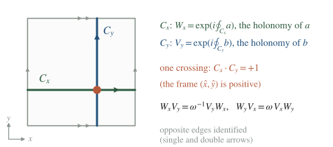
Figure 1. The torus with its two cycles. The holonomy of $a$ along $C_x$ and the holonomy of $b$ along $C_y$ meet at one point, and (3.5) assigns that point the commutator $2\pi i/N$.

3.4 $W^N=1$ and $\mathrm{GSD}(T^2)=N^2$

The relation (3.6) alone does not make the count finite: the determinant of both sides in dimension $n$ gives ${\omega }^n=1$, so its finite-dimensional unitary representations have dimensions divisible by $N$, and it also has infinite-dimensional ones (on $L^2$ of a noncompact variable). What makes the count finite is the compactness of $b$. By (3.3), $[{\oint }_{\gamma }a,b_j(\mathbf{y})]=\frac{2\pi i}{N}{\oint }_{\gamma }d{x}^i{ϵ}_{ij}{\delta }^2(\mathbf{x}-\mathbf{y})$, and therefore

$$W(\gamma {)}^N{b}_j(\mathbf{y})W(\gamma {)}^{-N}=b_j(\mathbf{y})+iN[{\oint }_{\gamma }a,b_j(\mathbf{y})]=b_j(\mathbf{y})-2\pi ({\delta }_{\gamma }{)}_j(\mathbf{y}),({\delta }_{\gamma }{)}_j(\mathbf{y})\equiv {\oint }_{\gamma }d{x}^i{ϵ}_{ij}{\delta }^2(\mathbf{x}-\mathbf{y}),\text{\hspace{1em}(3.8)}$$

where ${\delta }_{\gamma }$ is the Poincaré dual of γ: a closed 1-form with ${\oint }_{{\gamma }^{\prime }}{\delta }_{\gamma }=\gamma \cdot {\gamma }^{\prime }\in \mathbb{Z}$. So $W(\gamma {)}^N$ shifts $b$ by a closed form with periods in $2\pi \mathbb{Z}$, which is a large gauge transformation of $b$. The configurations it relates are the same $U(1)$ field, physical states are invariant under it, and $W(\gamma {)}^N=1$ on the physical space; by the exchange symmetry $V(\gamma {)}^N=1$ as well.

The physical space is irreducible under these operators, as the zero modes show. Modulo small gauge transformations, the solutions of (3.2) on $T^2$ are harmonic plus exact, $a={\theta }_{1}dx/L_x+{\theta }_{2}dy/L_y+d\lambda$ and $b={\phi }_{1}dx/L_x+{\phi }_{2}dy/L_y+d\tilde{\lambda }$, with ${\theta }_i={\oint }_{C_i}a$ and ${\phi }_i={\oint }_{C_i}b$, and the large gauge transformations shift each of ${\theta }_i$, ${\phi }_i$ by $2\pi$. Inserting them into (3.1), whose constraint terms now vanish,

$$S=\frac{N}{2\pi }\int dt({\phi }_2{\dot{\theta }}_1-{\phi }_1{\dot{\theta }}_2),\text{\hspace{1em}(3.9)}$$

two copies of $L=\frac{N}{2\pi }\phi \dot{\theta }$, consistent with (3.5): $[{\theta }_1,{\phi }_2]=2\pi i/N=-[{\theta }_2,{\phi }_1]$. In one copy the momentum of θ is $p=N\phi /2\pi$; the periodicity $\theta \sim \theta +2\pi$ quantizes $p\in \mathbb{Z}$; $e^{i\theta }$ raises $p$ by one, and $e^{i\phi }=e^{2\pi ip/N}={\omega }^p$ is diagonal. The large gauge transformation $\phi \to \phi +2\pi$ is the translation $p\to p+N$, so the physical states are labelled by $p$ mod $N$: there are $N$ of them, on which $e^{i\phi }$ and $e^{i\theta }$ act as clock and shift. Every function on the compact phase space is a Fourier series in $e^{i\theta }$ and $e^{i\phi }$, so these operators act irreducibly. With two copies,

$$\boxed{\mathrm{GSD}(T^2)=N^2,}\text{\hspace{1em}(3.10)}$$

the unique irreducible representation of the two pairs of (3.7) (Week 2 §8, one factor $N$ per pair). The same number is the symplectic area of each holonomy torus, $\frac{N}{2\pi }(2\pi {)}^2=2\pi N$, divided by $2\pi \hslash$, squared. It agrees with Week 14 (7.1) at $q\equiv 0$ and with Week 15 (3.3) at $N=2$, and enumeration of flat ${\mathbb{Z}}_N$ connections modulo gauge on the $2\times 2$ lattice torus gives $|Z^1|/|B^1|=32/8$, $243/27$, $1024/64$, that is 4, 9, 16 states for $N=2,3,4$ (and 4 on the $3\times 3$ torus for $N=2$). This also settles the two assumptions that Week 2 §8 left open: the physical algebra is generated by the holonomies of the two fields, by the zero-mode reduction, and its only relations are $W^N=V^N=1$, by (3.8).

4. Genus $g$: $N^{2g}$ from $H_1({\Sigma }_g,{\mathbb{Z}}_N)$ [Proved.]

Equations (3.3)–(3.8) are local or homological, so they hold on any closed oriented surface ${\Sigma }_g$, and the reduced phase space is the space of pairs of flat $U(1)$ connections modulo gauge, $U(1{)}^{2g}\times U(1{)}^{2g}$. Take a symplectic basis $A_i$, $B_i$ of $H_1({\Sigma }_g,\mathbb{Z})$ (Figure 2), with $A_i\cdot B_j={\delta }_{ij}$ and $A_i\cdot A_j=B_i\cdot B_j=0$, and define

$$Z_i=W(A_i),X_i=U(B_i),Z_i^{\prime }=W(B_i),X_i^{\prime }=U(-A_i)=U(A_i{)}^{†},i=1,\dots ,g.\text{\hspace{1em}(4.1)}$$

By (3.6), $Z_i{X}_j={\omega }^{A_i\cdot B_j}{X}_j{Z}_i={\omega }^{{\delta }_{ij}}{X}_j{Z}_i$ and $Z_i^{\prime }{X}_j^{\prime }={\omega }^{-B_i\cdot A_j}{X}_j^{\prime }{Z}_i^{\prime }={\omega }^{{\delta }_{ij}}{X}_j^{\prime }{Z}_i^{\prime }$, while $Z_i$ commutes with $X_j^{\prime }$ (because $A_i\cdot A_j=0$) and $Z_i^{\prime }$ with $X_j$ (because $B_i\cdot B_j=0$). Every holonomy is a product of these: for $\gamma ={\sum }_i(m_i{A}_i+n_i{B}_i)$ in homology, $W(\gamma )={\prod }_i{Z}_i^{m_i}{Z}_i^{\prime n_i}$ and $U(\gamma )={\prod }_i{X}_i^{\prime -m_i}{X}_i^{n_i}$. So we have $2g$ commuting clock–shift pairs with $Z^N=X^N=1$, the zero-mode reduction gives $2g$ copies of (3.9) and therefore irreducibility, and

$$\boxed{\mathrm{GSD}({\Sigma }_g)=N^{2g}=|H^1({\Sigma }_g,{\mathbb{Z}}_N)|,}\text{\hspace{1em}(4.2)}$$

one factor $N^2$ per handle, from the two pairs ($a$ on $A_i$ with $b$ on $B_i$, and $a$ on $B_i$ with $b$ on $A_i$). In the eigenbasis of the $W$‘s a state is labelled by $\alpha \in \mathrm{Hom}(H_1({\Sigma }_g),{\mathbb{Z}}_N)=H^1({\Sigma }_g,{\mathbb{Z}}_N)$, the ${\mathbb{Z}}_N$ holonomy of $a$ on every cycle. On the sphere there is one state. We checked the irreducibility numerically: the commutant of the generators is one-dimensional for $(N,g)=(3,1)$, $(4,1)$ and $(2,2)$.

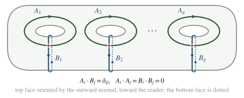
Figure 2. A symplectic basis of $H_1({\Sigma }_g)$, seen from above. $A_i$ runs around the $i$-th hole on the top face. $B_i$ runs on the top face (solid) from the rim of the $i$-th hole across $A_i$ to the outer edge and returns along the bottom face (dotted), so it goes once around the tube of the $i$-th handle. Only $A_i$ and $B_i$ intersect, once.

Euclidean check [Computed]. Since $H=0$, $Z({\Sigma }_g\times S^1)={\mathrm{Tr}}_{\mathcal{H}({\Sigma }_g)}{e}^{-\beta H}=\dim \mathcal{H}({\Sigma }_g)$. On a cellulation of $M$ with $N_0$ sites, $N_1$ links and $N_2$ plaquettes, take the dual presentation of §6.2, with $a\in C^1(M,{\mathbb{Z}}_N)$ on the links and $\tilde{b}$ on the $N_2$ dual links, one per plaquette. The normalized lattice BF partition function is

$$Z_{\mathrm{lat}}(M)=\frac{1}{N^{N_0+N_2}}\sum _{a,\tilde{b}}{\omega }^{⟨\tilde{b},\star da⟩}=\frac{|Z^1(M,{\mathbb{Z}}_N)|}{N^{N_0}}=\frac{|H^1(M,{\mathbb{Z}}_N)|}{|H^0(M,{\mathbb{Z}}_N)|},\text{\hspace{1em}(4.3)}$$

where the $\tilde{b}$-sum gives a factor $N$ times ${\delta }_{(da{)}_P,0}$ on every plaquette. On the cubic lattice links and plaquettes pair one to one, $N_1=N_2$, and (4.3) is the cup-product form $N^{-N_0-N_1}\sum {\omega }^{\sum b\cup da}$ of §6.2; on a general cellulation, such as a square-tiled ${\Sigma }_g\times S^1$, $N_1\ne N_2$ and only the dual form applies. As for the rest, and $|Z^1|=|H^1||B^1|$ with $|B^1|=N^{N_0}/|H^0|$. This is the normalization of an untwisted finite gauge theory by the volume of its gauge group, as in Dijkgraaf–Witten. For $M={\Sigma }_g\times S^1$ the Künneth formula gives $H^1={\mathbb{Z}}_N^{2g+1}$ and $H^0={\mathbb{Z}}_N$, so $Z=N^{2g}$, in agreement with (4.2); for $S^2\times S^1$, $Z=1$. On the cubic 3-tori with $L=2,3$ the rank of the coboundary matrices over ${\mathbb{F}}_N$ gives $|H^1|=N^3$ and $Z=N^2$ for $N=2,3$, and the genus-2 surface of Problem 3 gives $|H^1|=N^4$ for every subdivision we tried.

5. Braiding from linking in spacetime [Computed.]

5.1 The continuum computation

On $M=S^3$, let $C$ and $C^{\prime }$ be disjoint oriented closed curves, and define the Poincaré dual 2-form ${\delta }_C$ by ${\oint }_C\omega ={\int }_M\omega \wedge {\delta }_C$ for every 1-form ω (for $C^{\prime }$ the $z$-axis oriented upward, ${\delta }_{C^{\prime }}=\delta (x)\delta (y)dx\wedge dy$). Then

$$⟨W_e(C)V_m(C^{\prime })⟩=\frac{1}{Z}\int \mathcal{D}a\mathcal{D}b\exp (i{\int }_{M}b\wedge [\frac{N}{2\pi }da+m{\delta }_{C^{\prime }}]+ie{\int }_{M}a\wedge {\delta }_C).\text{\hspace{1em}(5.1)}$$

The $b$-integral is a δ-functional that imposes

$$da=-\frac{2\pi m}{N}{\delta }_{C^{\prime }},\text{\hspace{1em}(5.2)}$$

so the line $V_m(C^{\prime })$ is a thin tube of $a$-flux $-2\pi m/N$ along $C^{\prime }$. The solutions are $a=a_0+a_{\mathrm{flat}}$ with $a_0$ a particular solution; on $S^3$ a flat connection is pure gauge and drops out of $W_e(C)$ and of $Z$. Let $D$ be a Seifert surface, $\partial D=C$, oriented by Stokes’ theorem. Then

$${\oint }_C{a}_0={\int }_{D}d{a}_0=-\frac{2\pi m}{N}{\int }_D{\delta }_{C^{\prime }}=-\frac{2\pi m}{N}\mathrm{Lk}(C,C^{\prime }),\text{\hspace{1em}(5.3)}$$

where ${\int }_D{\delta }_{C^{\prime }}$ counts the crossings of $C^{\prime }$ through $D$, with $+1$ when $C^{\prime }$ crosses along the normal of $D$. This is the right-handed linking number: it equals the Gauss integral $\frac{1}{4\pi }\oint \oint \frac{(\mathbf{r}-{\mathbf{r}}^{\prime })\cdot (d\mathbf{r}\times d{\mathbf{r}}^{\prime })}{|\mathbf{r}-{\mathbf{r}}^{\prime }{|}^3}$, is symmetric in $C$ and $C^{\prime }$, and is $+1$ for a counterclockwise circle in the $xy$-plane and the $z$-axis oriented upward (Figure 3). Therefore

$$\boxed{⟨W_e(C)V_m(C^{\prime })⟩={\omega }^{-em\mathrm{Lk}(C,C^{\prime })}.}\text{\hspace{1em}(5.4)}$$

Integrating $a$ first gives $db=-\frac{2\pi e}{N}{\delta }_C$ and ${\oint }_{C^{\prime }}b=-\frac{2\pi e}{N}\mathrm{Lk}(C^{\prime },C)$, the same result, as the symmetry of Lk requires. The derivation shows which operator generates which symmetry: a $b$-line multiplies every linked $W_e(C)$ by a power of ω proportional to $e$, so it measures the electric charge and generates the electric ${\mathbb{Z}}_N^{(1)}$ of (2.4), while $W_s$ generates the magnetic one. With the generator $U_s=V_{-s}$ of §2.2,

$$⟨W_e(C)U_s(C^{\prime })⟩={\omega }^{es\mathrm{Link}(C,C^{\prime })},\mathrm{Link}=\mathrm{Lk},\text{\hspace{1em}(5.5)}$$

the Ward identity of conventions §6; §6.4 shows that the lattice definition of Link there is the right-handed linking number used here. The sign in $U_s=V_{-s}$ is forced by the sign of the weight: the line $V_m$ carries $a$-flux $-m$ by (5.2), so $U_s$ carries flux $+s$. The equal-time relation (3.6) is the same pairing seen in a time slice: two loops that cross once in space become linked once in spacetime when one of them is moved from just after to just before the other, which is the general relation between equal-time commutators and linking of Week 1 §6.3 (cross-reference: equal time from linking).

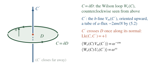
Figure 3. The linked pair of (5.4)–(5.5). The $b$-line pierces the Seifert disk of the Wilson loop once, and the $a$-flux $-2\pi m/N$ that it carries by (5.2) gives the Wilson loop its phase.

5.2 Anyons

Physical picture. In the Hamiltonian, an open line $W_e$ ends on two violations of $f_b=0$, the Gauss law of $a$: these are charges $\pm e$, the $e$ particles. An open line $U_{q^{\prime }}=V_{-q^{\prime }}$ ends on two violations of $f_a=0$: by (5.2) its endpoints carry $a$-flux $\pm q^{\prime }$ in units of $2\pi /N$, the $m$ particles. By (5.5), a charge $q=e$ carried once counterclockwise around a static flux $q^{\prime }$, a trajectory whose closed worldline links the flux worldline with $\mathrm{Link}=+1$, acquires ${\omega }^{q{q}^{\prime }}$: the Aharonov–Bohm phase of conventions §9, which is $-1$ for $N=2$, as in the toric code. This is exact in BF theory. That the $N^2$ anyon types $(e,m)\in {\mathbb{Z}}_N^2$ match the $N^2$ states of (3.10) is a forward reference: Block 3 (Week 8 and after) derives the correspondence. What a numerical experiment on the lattice model sees is the same phase in the interference of a charge transported around a plaquette that carries one unit of flux.

6. The lattice dictionary

6.1 From the ${\mathbb{Z}}_N$ Villain theory to BF [Computed; the approach to the limit Controlled to $O(e^{-2{\pi }^2\beta /N^2})$.]

Consider the ${\mathbb{Z}}_N$ Villain theory in $d=3$ (GLSS (C.19), whose integer field with its $N\mathbb{Z}$ gauge shifts is our ${\mathbb{Z}}_N$ cochain $a$),

$$Z_V=\sum _{a\in C^1(\Lambda ,{\mathbb{Z}}_N)}\prod _{P}f((da{)}_P),f(x)=\sum _{n\in \mathbb{Z}}\exp [-\frac{2{\pi }^2\beta }{N^2}(x-Nn{)}^2],\text{\hspace{1em}(6.1)}$$

which is the $U(1)$ Villain action $\frac{\beta }{2}\Vert dA-2\pi n{\Vert }^2$ of conventions §4 restricted to $A=2\pi a/N$. The function $f$ is $N$-periodic, so it has a discrete Fourier expansion $f(x)={\sum }_{k\in {\mathbb{Z}}_N}\hat{f}(k){\omega }^{kx}$. Combining $x\in {\mathbb{Z}}_N$ and $n\in \mathbb{Z}$ into $y=x-Nn\in \mathbb{Z}$ (note that ${\omega }^{-kx}={\omega }^{-ky}$), and using the Poisson identity of conventions §3 with $\alpha =2{\pi }^2\beta /N^2$,

$$\hat{f}(k)=\frac{1}{N}\sum _{y\in \mathbb{Z}}{e}^{-\alpha y^2}{\omega }^{-ky}=\frac{1}{N}[1+2e^{-2{\pi }^2\beta /N^2}\cos \frac{2\pi k}{N}+O(e^{-8{\pi }^2\beta /N^2}\left)\right]=\frac{1}{\sqrt{2\pi \beta }}\sum _{w\in \mathbb{Z}}{e}^{-(Nw+k{)}^2/2\beta },\text{\hspace{1em}(6.2)}$$

where the middle form is the exact sum over $y$, which at large β is dominated by its first terms, and the last, from ${\sum }_y{e}^{-\alpha y^2}{e}^{-2\pi iky/N}=\sqrt{\pi /\alpha }{\sum }_w{e}^{-{\pi }^2(w-k/N{)}^2/\alpha }$ with ${\pi }^2/\alpha =N^2/2\beta$, is a Villain weight of coupling $1/\beta$ for the dual variable, GLSS (C.23). The exact sum and the dual form agree to machine precision for $(N,\beta )=(3,0.7)$, $(4,2)$ and $(5,5)$. Inserting the expansion plaquette by plaquette,

$$Z_V=\sum _a\sum _{k\in C^2(\Lambda ,{\mathbb{Z}}_N)}[\prod _P\hat{f}(k_P)]{\omega }^{⟨k,da⟩}=\sum _a\sum _{\tilde{b}\in C^1({\Lambda }^{\ast },{\mathbb{Z}}_N)}[\prod _{\tilde{\ell }}\hat{f}({\tilde{b}}_{\tilde{\ell }})]{\omega }^{⟨\tilde{b},\star da{⟩}_{{\Lambda }^{\ast }}},\text{\hspace{1em}(6.3)}$$

where $\tilde{b}\equiv \star k$, and $⟨k,da⟩=⟨\star k,\star da⟩$ because the Hodge map of conventions §2 moves values with signs $\pm 1$. The field $\tilde{b}$ on dual links is the Fourier label of the plaquette weight, the electric flux: summing over $a$ imposes $\delta k=0$, which is $d\tilde{b}=0$ because $\delta =\star d\star$ on $C^2$ in $d=3$ (checked cell by cell), the ${\mathbb{Z}}_N$ version of the conserved Hubbard–Stratonovich integer of Week 8 (conventions §5). The weight of a flux configuration relative to zero flux is

$$\frac{\hat{f}(k)}{\hat{f}(0)}=1-2(1-\cos \frac{2\pi k}{N})e^{-2{\pi }^2\beta /N^2}+O\left(e^{-4{\pi }^2\beta /N^2}\right),\text{\hspace{1em}(6.4)}$$

the Boltzmann factor of the electric energy. At zero coupling, β = ∞, every $\hat{f}(k)\to 1/N$, and

$$Z_V{|}_{\beta =\infty }=\frac{1}{N^{N_P}}\sum _{a\in C^1(\Lambda ,{\mathbb{Z}}_N)}\sum _{\tilde{b}\in C^1({\Lambda }^{\ast },{\mathbb{Z}}_N)}{\omega }^{⟨\tilde{b},\star da{⟩}_{{\Lambda }^{\ast }}}.\text{\hspace{1em}(6.5)}$$

Thus the lattice BF theory is ${\mathbb{Z}}_N$ lattice gauge theory at zero coupling, with the electric flux promoted to a field of its own, and the corrections at large β are controlled by the one-flux suppression $e^{-2{\pi }^2\beta /N^2}$. The Wilson plaquette weight gives the same limit (Problem 2).

6.2 From the dual lattice to the cup product, and the GLSS presentation [Computed.]

Write ${\Lambda }^{\ast }=\Lambda +h$ with $h=\frac{1}{2}(1,1,1)$, and label the cell of ${\Lambda }^{\ast }$ based at $y+h$ with directions $T$ by $(y;T)$. The duality rule of conventions §2 then reads $(x;S{)}^{\ast }=(x-{\hat{e}}_{S^c};S^c)$ and $(y;T{)}^{\ast }=(y+{\hat{e}}_T;T^c)$. For $b\in C^1(\Lambda ,{\mathbb{Z}}_N)$ define $\tilde{b}\in C^1({\Lambda }^{\ast },{\mathbb{Z}}_N)$ by $\tilde{b}(y;\mu )=b_{\mu }(y)$. The cubical cup product of conventions §8 on a cube has three terms,

$$(b\cup da)(x;123)=b_1(x)(da{)}_{23}(x+\hat{1})-b_2(x)(da{)}_{13}(x+\hat{2})+b_3(x)(da{)}_{12}(x+\hat{3}),\text{\hspace{1em}(6.6)}$$

so each $b_{\mu }(x)$ multiplies exactly one plaquette, $P_{S^c}(x+\hat{\mu })$ with $S^c$ the complement of μ. That plaquette is the dual of the ${\Lambda }^{\ast }$-link $(x;\mu )$, since its dual is based at $x+\hat{\mu }-\hat{\mu }+h$ in direction μ, and the cup sign $ϵ(\{\mu \},S^c)$ equals the Hodge sign $ϵ(S^c,\{\mu \})$, because moving one index past two is an even permutation. Summing over cubes,

$$\boxed{\sum _{\mathrm{cubes}}b\cup da=⟨\tilde{b},\star da{⟩}_{{\Lambda }^{\ast }}=⟨a,\star d\tilde{b}{⟩}_{\Lambda },}\text{\hspace{1em}(6.7)}$$

where the second equality is summation by parts between Λ and ${\Lambda }^{\ast }$, the lattice form of $\int b\wedge da=\int a\wedge db$. We checked both equalities exactly on random integer cochains on $3^3$ and $4^3$ tori, and checked that ${\ell }_{\mu }(x)\mapsto P_{S^c}(x+\hat{\mu })$ is a bijection between links and plaquettes (Figure 4). Three consequences follow.

(a) The normalization (4.3). On the cubic lattice, where links and plaquettes pair one to one, the sum over $b\in C^1(\Lambda ,{\mathbb{Z}}_N)$ gives $N^{N_1}{\prod }_P{\delta }_{(da{)}_P,0}$, each plaquette constrained exactly once.

(b) The ordering of the cup product. With the factors exchanged, $da$ sits at the base corner and $b$ at the far corner, and

$$\sum _{\mathrm{cubes}}da\cup b[b]=\sum _{\mathrm{cubes}}b\cup da[Tb],(Tb{)}_{\mu }(x)=b_{\mu }(x+(1,1,1)),\text{\hspace{1em}(6.8)}$$

which we also checked; by the Leibniz rule of conventions §8 the left side equals $\sum a\cup db$. The ordering $b\cup da$ puts $b$ on $\Lambda +h$ and the ordering $a\cup db$ puts it on $\Lambda -h$: two copies of the dual lattice related by a translation, which on a torus relabels the summation variable. The two orderings define the same theory, while pointwise they differ (§9.4).

(c) The GLSS presentation. GLSS write the β → ∞ limit of (C.19) as the weight $e^{-S}$ with $S=\frac{2\pi i}{N}{\sum }_{p\text{-cell}}m\Delta \tilde{n}$, their (C.21), which at $p=1$, $d=3$ has integers $m$ on links and $\tilde{n}$ on dual links, with the gauge symmetries (C.20) and (C.22) that include the shifts by $N\mathbb{Z}$. Their pairing of a link with its dual plaquette is our $\star$, up to their orientation convention for dual cells; with $m=a$ and $\tilde{n}=-\tilde{b}$, the sign absorbing $e^{-S}$, (C.21) is the last expression in (6.7). Read from right to left, (6.7) turns the GLSS presentation into the cup form of conventions §7; read from left to right, it removes the cup product in favour of $\tilde{b}$ on ${\Lambda }^{\ast }$. [GLSS’s equations: Stated — refs: GLSS App. C.2.]

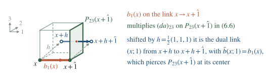
Figure 4. Why the cup product is a dual-lattice pairing: the link that carries $b_1(x)$, shifted by $h$, is the dual link through the plaquette $P_{23}(x+\hat{1})$ that $b_1(x)$ multiplies in (6.6).

6.3 From the lattice to the continuum and back [Computed; the continuum limit Stated — refs: GLSS (C.31)–(C.33).]

Lattice to continuum. Set $A_{\ell }=\frac{2\pi }{N}{a}_{\ell }$ and $B_{\tilde{\ell }}=\frac{2\pi }{N}{\tilde{b}}_{\tilde{\ell }}$. Then

$$\frac{2\pi i}{N}⟨\tilde{b},\star da⟩=\frac{iN}{2\pi }⟨B,\star dA⟩,\text{\hspace{1em}(6.9)}$$

where $⟨B,\star dA⟩$ is the lattice transcription of $\int B\wedge dA$ (the pairing $⟨\alpha ,\star \beta ⟩$ transcribes $\int \alpha \wedge \beta$, with $\star \star =1$ in $d=3$), and the flatness $da\equiv 0$ mod $N$ becomes $dA\in 2\pi C^2(\Lambda ,\mathbb{Z})$: $A$ is a $U(1)$ lattice connection with vanishing Villain field strength and ${\mathbb{Z}}_N$ holonomies. The integrality (2.2) is automatic on the lattice: $\tilde{b}\to \tilde{b}+N$ on one dual link changes the exponent by $2\pi i(\star da{)}_{\tilde{\ell }}\in 2\pi i\mathbb{Z}$.

Continuum to lattice. The continuum fields are $U(1)$ gauge fields, and the lattice carries this structure with three ingredients: real cochains $a\in C^1(\Lambda ,\mathbb{R})$ and $\tilde{b}\in C^1({\Lambda }^{\ast },\mathbb{R})$; Villain integers $n\in C^2(\Lambda ,\mathbb{Z})$ and $\tilde{n}\in C^2({\Lambda }^{\ast },\mathbb{Z})$ that make them compact; and Stueckelberg fields $\varphi \in C^0(\Lambda ,\mathbb{R})$ and $\tilde{\varphi }\in C^0({\Lambda }^{\ast },\mathbb{R})$ that keep the real gauge symmetry exact. The weight is

$$\mathcal{W}=\exp \{\frac{iN}{2\pi }⟨\tilde{b},\star da{⟩}_{{\Lambda }^{\ast }}-i⟨\tilde{n},\star (Na-d\varphi ){⟩}_{{\Lambda }^{\ast }}-i⟨N\tilde{b}-d\tilde{\varphi },\star n{⟩}_{{\Lambda }^{\ast }}\},\text{\hspace{1em}(6.10)}$$

and it is invariant under

$$\begin{array}{rlrl}& \text{(i)}a\to a+d\lambda ,\varphi \to \varphi +N\lambda ;& & \text{(ii)}\tilde{b}\to \tilde{b}+d\tilde{\lambda },\tilde{\varphi }\to \tilde{\varphi }+N\tilde{\lambda };\\ & \text{(iii)}a\to a+2\pi k,n\to n+dk;& & \text{(iv)}\tilde{b}\to \tilde{b}+2\pi \tilde{k},\tilde{n}\to \tilde{n}+d\tilde{k};\\ & \text{(v)}\varphi \to \varphi +2\pi k_{\varphi };& & \text{(vi)}\tilde{\varphi }\to \tilde{\varphi }+2\pi {\tilde{k}}_{\varphi },\end{array}\text{\hspace{1em}(6.11)}$$

with λ, $\tilde{\lambda }$ real and $k,\tilde{k},k_{\varphi },{\tilde{k}}_{\varphi }$ integer cochains. In (i) and (ii) the combinations $Na-d\varphi$ and $N\tilde{b}-d\tilde{\varphi }$ are invariant, and the first term changes only in (ii), by $\frac{iN}{2\pi }⟨d\tilde{\lambda },\star da⟩=\frac{iN}{2\pi }⟨a,\star dd\tilde{\lambda }⟩=0$ by (6.7). Under (iii) the first term changes by $iN⟨\tilde{b},\star dk⟩$, the second by $-2\pi iN⟨\tilde{n},\star k⟩\in 2\pi i\mathbb{Z}$, and the third by $-iN⟨\tilde{b},\star dk⟩+i⟨d\tilde{\varphi },\star dk⟩$; the total is $i⟨d\tilde{\varphi },\star dk⟩=i⟨k,\star dd\tilde{\varphi }⟩=0$ by (6.7). Under (iv) the first term changes by $iN⟨\tilde{k},\star da⟩$, the second by $-iN⟨d\tilde{k},\star a⟩+i⟨d\tilde{k},\star d\varphi ⟩$, and the third by $-2\pi iN⟨\tilde{k},\star n⟩\in 2\pi i\mathbb{Z}$. In $d=3$ the pairings $⟨g,\star f{⟩}_{{\Lambda }^{\ast }}$ and $⟨f,\star g{⟩}_{\Lambda }$ coincide (the shuffle signs of a 2-set and its complement agree), so $⟨d\tilde{k},\star a⟩=⟨a,\star d\tilde{k}⟩=⟨\tilde{k},\star da⟩$ by (6.7), and the first two changes cancel, while $⟨d\tilde{k},\star d\varphi ⟩=⟨\tilde{k},\star dd\varphi ⟩=0$. Changes (v) and (vi) are in $2\pi i\mathbb{Z}$. We checked all six numerically on the $3^3$ torus with $N=5$: the real transformations leave the exponent unchanged to $10^{-14}$, and the integer ones change it by $2\pi$ times an integer to the same accuracy. Up to orientation conventions, (6.10) is GLSS (C.26) at $p=1$, $d=3$ after $(\tilde{b},\tilde{m},\tilde{\varphi }{)}_{\mathrm{GLSS}}=-(\tilde{b},\tilde{n},\tilde{\varphi })$.

The reduction to ${\mathbb{Z}}_N$ cochains takes three lines. The sum over $\tilde{n}\in C^2({\Lambda }^{\ast },\mathbb{Z})$ is a product over links of ${\sum }_{\tilde{n}}{e}^{-i\tilde{n}x}=2\pi {\sum }_m\delta (x-2\pi m)$, and the sum over $n$ is the same over dual links, so

$$a=\frac{d\varphi +2\pi m}{N},\tilde{b}=\frac{d\tilde{\varphi }+2\pi \tilde{m}}{N},m\in C^1(\Lambda ,\mathbb{Z}),\tilde{m}\in C^1({\Lambda }^{\ast },\mathbb{Z}).\text{\hspace{1em}(6.12)}$$

The gauge choice $\varphi =\tilde{\varphi }=0$ uses up (i) and (ii); the residual transformations (iii) and (iv) shift $m$ and $\tilde{m}$ by $N$ times integers, so $m$ and $\tilde{m}$ are ${\mathbb{Z}}_N$ cochains; and the first term of (6.10) becomes $\frac{iN}{2\pi }(\frac{2\pi }{N}{)}^2⟨\tilde{m},\star dm⟩=\frac{2\pi i}{N}⟨\tilde{m},\star dm⟩$, which is (6.5) and, by (6.7), the cup form of conventions §7. (Before gauge fixing, the cross term $\frac{1}{N}⟨d\tilde{\varphi },\star dm⟩$ vanishes by (6.7); we checked the reduced weight numerically as well.) Thus the continuum theory, put on the lattice with its gauge structure intact, is the ${\mathbb{Z}}_N$ lattice BF theory with the same integer $N$, and in the gauge where $n$ and $\tilde{n}$ vanish except on the few cells that carry the transition functions, (6.10) tends to (2.1) as the lattice spacing goes to zero [Stated — refs: GLSS (C.31)–(C.33)].

The Stueckelberg combination has a physical reading. Since ${\sum }_m{e}^{-\frac{\kappa }{2}(x-2\pi m{)}^2}=(2\pi \kappa {)}^{-1/2}{\sum }_{\tilde{n}}{e}^{-{\tilde{n}}^2/2\kappa +i\tilde{n}x}$ (conventions §3), the term $-i⟨\tilde{n},\star (Na-d\varphi )⟩$ summed over $\tilde{n}$ is the κ → ∞ limit of a Villain coupling of a charge-$N$ Higgs field φ: BF theory is $U(1)$ Higgsed to ${\mathbb{Z}}_N$ in the London limit, which is Kapustin–Seiberg (3.7)–(3.9) on the lattice, the $U(1)$ version of the κ = ∞ edge of Week 14 §2, and, at $N=2$, the superconductor of Week 14 §8.

6.4 The Hamiltonian dictionary and the lattice linking [Computed.]

On the spatial square lattice each link carries ${\mathbb{C}}^N$ with $Z|k⟩={\omega }^k|k⟩$, $X|k⟩=|k+1⟩$ and $ZX=\omega XZ$ (Week 2 §8). By (3.5), the integrals of $a$ over a link ℓ and of $b$ over the dual link $\tilde{\ell }$ that crosses it with $\ell \cdot \tilde{\ell }=+1$ obey $[{\int }_{\ell }a,{\int }_{\tilde{\ell }}b]=2\pi i/N$, so with $e^{i{\int }_{\ell }a}\leftrightarrow Z_{\ell }$ we need $Z_{\ell }{e}^{i{\int }_{\tilde{\ell }}b}={\omega }^{-1}{e}^{i{\int }_{\tilde{\ell }}b}{Z}_{\ell }$, that is,

$$e^{i{\int }_{\tilde{\ell }}b}⟷X_{\ell }^{†},W(\gamma )\leftrightarrow \prod _{\ell \in \gamma }{Z}_{\ell }^{\pm 1},U(\tilde{\gamma })=V(\tilde{\gamma }{)}^{†}\leftrightarrow \prod _{\ell ⋔\tilde{\gamma }}{X}_{\ell }^{\ell \cdot \tilde{\gamma }},\text{\hspace{1em}(6.13)}$$

with the exponent $+1$ in $W$ for links traversed along their orientation. The generator of the electric symmetry is thus the string of shift operators $X$ on the links that $\tilde{\gamma }$ crosses positively, and a Wilson string and a generator string that share one such link obey $WU=\omega UW$, which is $ZX=\omega XZ$ on that link and (3.6) on the torus. The constraints (3.2) become the plaquette and star conditions. The $a$-holonomy around a plaquette is $B_P={\prod }_{\partial P}Z$, so $f_a=0$ is $B_P=1$. The $b$-holonomy around the small counterclockwise dual loop that encircles a site $x$ crosses each outgoing link with $\ell \cdot \tilde{\gamma }=+1$ and each incoming one with $-1$, so it equals ${\prod }_i{X}_{(x-\hat{i},i)}{X}_{(x,i)}^{†}=G_x$, and $f_b=0$ is Gauss’s law $G_x=1$ of conventions §4. The BF Hilbert space on $T^2$ is therefore the ground space of $-{\sum }_x\mathrm{Re}{G}_x-{\sum }_P\mathrm{Re}{B}_P$, the $\Gamma \to 0$ point of the ${\mathbb{Z}}_N$ Kogut–Susskind Hamiltonian with the Gauss law imposed energetically (Week 7 §8 for $N=2$; Week 14 §7.1 at $q\equiv 0$, where the explicit $9\times 9$ ground-space matrices of the holonomies for $N=3$ were computed). The electric-flux operator $U_i(n)={\prod }_{x_i=n}{X}_{(x,i)}$ of conventions §4 is $U(\tilde{\gamma })$ for the dual curve that crosses that column positively, and for $N=2$ the dictionary is Week 15 §3.4, where $W_i=\prod {\sigma }^z$, $U_i=\prod {\sigma }^x$, and (3.2) there is (3.7) here. Figure 5 shows the two strings and their single shared link.

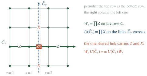
Figure 5. The lattice holonomies of (6.13) on a spatial torus. The Wilson string of $Z$‘s along $C_x$ and the string of $X$‘s on the links crossed by the dual curve ${\tilde{C}}_y$ share one link, which carries the single factor of ω in (3.7).

The lattice linking. The generator $U_s(\tilde{c})$ of conventions §6 replaces $(da{)}_P$ by $(da{)}_P-s$ on the plaquettes dual to a closed dual curve $\tilde{c}=\partial \tilde{V}$, oriented so that $d{\lambda }_{\tilde{V}}=+1$ on them, where ${\lambda }_{\tilde{V}}$ is the signed indicator of the links dual to the cells of $\tilde{V}$. With the Hodge orientations of conventions §2, ${\lambda }_{\tilde{V}}=\star 1_{\tilde{V}}$, and $d{\lambda }_{\tilde{V}}=\star 1_{\tilde{c}}$ follows from $1_{\partial \tilde{V}}=\delta 1_{\tilde{V}}$ and $\delta =\star d\star$ on $C^2({\Lambda }^{\ast })$, which we checked. By the Fourier expansion of §6.1, $f((da{)}_P-s)={\sum }_k\hat{f}(k){\omega }^{k(da{)}_P}{\omega }^{-ks}$, so the replacement inserts ${\omega }^{-s⟨\tilde{b},1_{\tilde{c}}⟩}$, with $1_{\tilde{c}}$ the indicator cochain of $\tilde{c}$:

$$U_s(\tilde{c})=\exp (-\frac{2\pi is}{N}\sum _{\tilde{c}}\tilde{b})=V_{-s}(\tilde{c})\text{at every }\beta ,\text{\hspace{1em}(6.14)}$$

the lattice form of the generator of §2.2. The symmetry operator of the lattice gauge theory is a $b$-line, so $b$ was present in the Wilson and Villain theories from the start. In the BF theory the sum over $\tilde{b}$ in $⟨W_e(C)U_s(\tilde{c})⟩$ imposes $\star da-s{1}_{\tilde{c}}\equiv 0$, that is $da=sd{\lambda }_{\tilde{V}}$; the solutions are $a=a^{\prime }+s{\lambda }_{\tilde{V}}$ with $a^{\prime }$ flat, and $W_e(C)={\omega }^{e{\sum }_{C}a}$ acquires ${\omega }^{es⟨J_C,{\lambda }_{\tilde{V}}⟩}$, where $\mathrm{Link}(C,\partial \tilde{V})\equiv ⟨J_C,{\lambda }_{\tilde{V}}⟩=\#(C\cap \tilde{V})$ is the definition of conventions §6. For four configurations on the cubic lattice (a plaquette loop with a dual loop through it in both orientations, a $2\times 1$ loop, and an unlinked pair) we computed $⟨J_C,{\lambda }_{\tilde{V}}⟩=-1,+1,-1,0$ and the Gauss integral of the embedded curves, which agrees in every case: the lattice Link is the right-handed linking number of §5.1 (for the lattice pairing in general, Week 1 §5.1, cross-reference). The BF phases are ${\omega }^{-1},{\omega }^{+1},{\omega }^{-1},1$ for $e=s=1$. Therefore

$$⟨W_e(C)U_s(\tilde{c})⟩={\omega }^{es\mathrm{Link}(C,\tilde{c})}⟨W_e(C)⟩,\text{\hspace{1em}(6.15)}$$

the lattice face of (5.5). The change of variables never uses β = ∞, so (6.15) holds at every β of the pure gauge theory: it is the Ward identity of conventions §6 and of Week 14 (3.2).

7. Degeneracy as spontaneously broken 1-form symmetry

7.1 The symmetry permutes the ground states [Proved.]

On the spatial $T^2$ the electric ${\mathbb{Z}}_N^{(1)}$ is represented by the generators $U(\tilde{\gamma })$ on closed curves, which are topological on the physical space by (3.2); wrapped on the two cycles they form the group $\{U(\tilde{\gamma })\}\cong H_1(T^2,{\mathbb{Z}}_N)\cong {\mathbb{Z}}_N^2$, which acts on the Hilbert space as an ordinary symmetry. The charged objects are the $W(\gamma )$. In the holonomy basis $W(\gamma )|\alpha ⟩={\omega }^{\alpha (\gamma )}|\alpha ⟩$, $\alpha \in H^1(T^2,{\mathbb{Z}}_N)$, and (3.6) gives $W(\gamma )U(\tilde{\gamma })|\alpha ⟩={\omega }^{\alpha (\gamma )+\gamma \cdot \tilde{\gamma }}U(\tilde{\gamma })|\alpha ⟩$, so that, with the phases fixed by $|{\alpha }_1,{\alpha }_2⟩=X_1^{{\alpha }_1}{X}_2^{{\alpha }_2}|0,0⟩$ in the notation of (3.7),

$$U(\tilde{\gamma })|\alpha ⟩=|\alpha +{\iota }_{\tilde{\gamma }}⟩,{\iota }_{\tilde{\gamma }}(\gamma )\equiv \gamma \cdot \tilde{\gamma }.\text{\hspace{1em}(7.1)}$$

By Poincaré duality $\tilde{\gamma }\mapsto {\iota }_{\tilde{\gamma }}$ is an isomorphism $H_1(T^2,{\mathbb{Z}}_N)\to H^1(T^2,{\mathbb{Z}}_N)$, so the symmetry acts on the $N^2$ states $|\alpha ⟩$ by translations of $H^1$, freely and transitively, and no $|\alpha ⟩$ is invariant. This is the structure of a ferromagnet with $N^2$ ordered states that a global symmetry permutes, with the Wilson loops in the role of the magnetization.

7.2 Clustering selects the broken states [Proved.]

Two questions remain: which ground states play the role of the ordered states, and what the order parameter does. Let γ and γ′ be disjoint homologous cycles, for instance $C_x$ at $y=0$ and at $y=L_y/2$. On the physical space $W({\gamma }^{\prime })=W(\gamma )$ (§3.3), so in every ground state ψ

$$⟨\psi |W(\gamma )W({\gamma }^{\prime }{)}^{†}|\psi ⟩-⟨\psi |W(\gamma )|\psi ⟩⟨\psi |W({\gamma }^{\prime }{)}^{†}|\psi ⟩=1-|⟨\psi |W(\gamma )|\psi ⟩{|}^2,\text{\hspace{1em}(7.2)}$$

independent of the separation: the order parameter has long-range order in every ground state. The connected part vanishes, which is the clustering of the order parameter, if and only if $|⟨\psi |W(\gamma )|\psi ⟩|=1$, which for a unitary operator means that ψ is an eigenvector of $W(\gamma )$ (the Cauchy–Schwarz inequality is saturated). Requiring this for $C_x$ and $C_y$ selects the joint eigenvectors of $W_x$ and $W_y$, and each of the $N^2$ joint eigenvalues occurs once, so the clustering states are exactly the $|\alpha ⟩$. In them the order parameter is nonzero, $|⟨W⟩|=1$, and by (7.1) the symmetry permutes them: the electric ${\mathbb{Z}}_N^{(1)}$ is spontaneously broken. The symmetric states, eigenstates of $U(C_x)$ and $U(C_y)$, have $⟨W(\gamma )⟩=0$ and do not cluster, like the symmetric superposition of the two Ising ground states. For contractible loops the $b$-integral gives $da=0$, and therefore

$$⟨W_e(C)⟩=1(C\text{contractible}),\text{\hspace{1em}(7.3)}$$

a perimeter law with zero perimeter coefficient: the criterion of conventions §6 for a broken 1-form symmetry, in its strongest form. By the exchange symmetry, the same argument with $a\leftrightarrow b$ shows that the magnetic ${\mathbb{Z}}_N^{(1)}$, generated by the $W$‘s, is broken with order parameter $V$, and that its clustering states are the eigenstates of $V_x$ and $V_y$. The two selections are incompatible, since $W_x$ and $V_y$ do not commute: no ground state clusters for both order parameters at once. In the lattice theory away from its soluble point only the electric symmetry is exact (§9.5), its order parameter is $W$, and the selection is the first one.

7.3 Breaking forces degeneracy, and the unbroken case [Proved at the soluble points; Sketched in between.]

The algebra of §3 forces the degeneracy whenever the symmetry is broken. On the lattice, $U(\tilde{\gamma })$ commutes with the Hamiltonian at every coupling, and $W(\gamma )U(\tilde{\gamma })={\omega }^{c}U(\tilde{\gamma })W(\gamma )$ holds as an operator identity, $c=\gamma \cdot \tilde{\gamma }$, because each link the two strings share contributes ${\omega }^{\pm 1}$ by (6.13), with net exponent $c$. If $P$ projects onto the low-lying states, $[U,P]=0$, and

$$(PWP)U=PWUP={\omega }^{c}PUWP={\omega }^{c}U(PWP).\text{\hspace{1em}(7.4)}$$

So $PWP$ maps an eigenvector of $U$ with eigenvalue $u$ to one with eigenvalue ${\omega }^{-c}u$ or to zero. When the wrapped Wilson loop acts invertibly on the low-lying states, which is the operator content of a perimeter law (in the deconfined phase $PWP$ is a nonzero multiple of a unitary up to corrections that vanish as $L\to \infty$), the low-lying space contains $N$ eigenvalues of $U$ per conjugate pair: at least $N^2$ states, split by an amount exponentially small in $L$ (Week 14 §7.2). When the symmetry is unbroken (area law), $W(\gamma )$ creates a loop of electric flux whose energy grows with $L$, $PWP\to 0$, and nothing forces a degeneracy: at the confined soluble point $K=0$ the ground state is unique and has $U=1$ (Week 15 §3.4). Week 3 turns this dichotomy into the general criterion; here it is exact at the two soluble points.

7.4 Both symmetries, and their mutual charges [Stated — forward references.]

In BF theory each symmetry’s generators are the other’s charged objects, (3.6) and (5.4). The incompatibility found at the end of §7.2 is the finite-volume face of a mixed ‘t Hooft anomaly between the electric and magnetic ${\mathbb{Z}}_N^{(1)}$: wherever both are present, a symmetric, gapped, non-degenerate ground state on the torus is impossible (Block 2, skeleton). Gauging one of them, by summing over the insertions of its generators, is the subject of Week 4. In the lattice model the magnetic symmetry is exact only at the soluble point, and it emerges at long distances in the deconfined phase (conventions §6, “Lattice versus TQFT”).

Physical picture. In a Monte Carlo simulation of three-dimensional ${\mathbb{Z}}_N$ lattice gauge theory on an $L^3$ torus, measure the correlator of two Wilson lines that wind the same cycle of one time slice at separation $s$. In the deconfined phase it depends on $L$ through the perimeter factor and is independent of $s$, the long-range order of (7.2); in the confined phase it decays as $e^{-\sigma Ls}$, the area of the strip between the lines. At β = ∞ flatness makes all parallel lines equal configuration by configuration, which is (7.2) exactly; at finite β the statement is the perimeter and area laws of Week 5 §§4–5 [Heuristic for the size of the corrections]. The SSB reading thus predicts something measurable: the degeneracy of §3 is the long-range order of wrapped lines, and it disappears where the area law sets in.

8. Seminar: the Kogut–Susskind ${\mathbb{Z}}_2$ theory is the toric code

Paper and sections. Kitaev, quant-ph/9707021, the sections on toric codes and the corresponding Hamiltonians, on abelian anyons, and the first part of the section on materialized symmetry (§§1–3 of the arXiv text), about 15 minutes of presentation for §2 and 10 each for §§3–4.

The technical claim. The protected subspace of the toric code on a $k\times k$ torus, on which every star operator $A_s$ and plaquette operator $B_p$ equals one, is four-dimensional; the algebra of operators on it is generated by the products $Z_1,Z_2$ of ${\sigma }^z$ along two non-contractible loops and $X_1,X_2$ of ${\sigma }^x$ along two non-contractible cuts, with the commutation relations of two qubits; the excitations are created at the ends of string operators and braid with phase $-1$.

What it needs from Semester I. The ${\mathbb{Z}}_2$ Kogut–Susskind Hamiltonian, its flux sectors on the torus and the energetic Gauss law (Week 7 §§7.1, 7.4 and 8); $H^1(T^2,{\mathbb{Z}}_2)$ and the intersection pairing (Week 2 §§4.3 and 8); the translation exercise of Week 15 §3.4. In this dictionary $A_s$ is the Gauss-law operator, $B_p$ the plaquette term, the loops $Z_i$ the Wilson loops $W$, and the cuts $X_i$ the electric-flux operators $U_i$, which are the generators $U$ of (6.13).

The step at the board. Kitaev’s second computation of $\dim L=4$: the operators on $L$ form the commutant of the stabilizers modulo the ideal they generate; a contractible loop or cut is a product of $B_p$‘s or $A_s$‘s and therefore equals one modulo the ideal; so only the four non-contractible operators survive, and their commutation relations are those of ${\sigma }_1^z,{\sigma }_2^z,{\sigma }_1^x,{\sigma }_2^x$. The presenter then does the mini-step of the week: the same argument with ${\mathbb{Z}}_N$ clock and shift operators on ${\Sigma }_g$, giving $N^{2g}$ from $H_1({\Sigma }_g,{\mathbb{Z}}_N)$ and the intersection pairing, in full for $g=1$ and handle by handle beyond, which is §4 in lattice language.

Discussion and the open problem. Kitaev’s §4 reads the model as a ${\mathbb{Z}}_2$ gauge theory whose Gauss law is energetically favoured but not imposed, and finds a ${\mathbb{Z}}_2\times {\mathbb{Z}}_2$ symmetry “dynamically created” at long distances, behind the conservation of electric and magnetic charge modulo 2; he then asks what this symmetry is. In the language of this week it is the pair of 1-form symmetries of §7, both exact at the soluble point, the electric one exact at every coupling once the Gauss law is imposed as a constraint, and the magnetic one emergent. The instructor closes by placing the result on the course map: the deconfined phase of Week 5 is this code, Block 3 (Week 8) solves it, and Week 3 states the general SSB criterion that §7 derived in this model.

9. Subtleties and fine print

9.1 The global definition of the action. For $U(1)$ fields with fluxes, $b\wedge da$ is not the wedge product of globally defined forms, and ${\int }_{M}b\wedge da$ is defined with the transition functions of both fields (Deligne–Beilinson cocycles, Kapustin–Seiberg §3). The identity $\int b\wedge da=\int a\wedge db$ and the computation (2.2) hold in that framework. The lattice presentations need no such care: in (6.5) and (6.7) the fields are cochains and the level is automatically an integer (§6.3); in (6.10) the transition functions are the Villain integers.

9.2 Compactness and large gauge invariance. Every finite number in this note comes from the identification of $\oint a$ and $\oint b$ modulo $2\pi$. The noncompact BF theory, with $\mathbb{R}$-valued fields, has the same bracket (3.3) and the same relation (3.6), but no relation $W^N=1$: its zero-mode Hilbert space is $L^2({\mathbb{R}}^2)$ and it has no ground-state degeneracy in any useful sense. On the lattice, compactness is the statement that $a$ and $\tilde{b}$ are ${\mathbb{Z}}_N$-valued, or, in (6.10), that the Villain integers are summed.

9.3 Orientation and the sign of the phase. The sign of $U_s=V_{-s}$ is fixed in §5.1. Reversing the orientation of spacetime changes the signs of $N$ and of Link together. In the $e^{-S}$ convention of GLSS and Kapustin–Seiberg the field $b$ is minus ours, so their natural $b$-line of charge $s$ is our $U_s$, and their phase carries the plus sign. A formula imported from a source is translated before use; the anyon statement of §5.2 needs no translation once the vortex is labelled by its flux.

9.4 Point splitting on the lattice. An $a$-line on links of Λ and a $b$-line on links of the same lattice can share links, and then their linking number is undefined. The cup product resolves this by placing $b$ on the shifted lattice $\Lambda +h$ (6.7), a lattice framing; the other ordering uses $\Lambda -h$ (6.8). Pointwise, $b\cup da$ and $da\cup b$ are different cochains, as the noncommutativity of the cup product of conventions §8 requires; on a torus the two theories are related by a translation, and they become different only in constructions sensitive to framing, such as self-linking and the twisted theories of Block 2.

9.5 Zero coupling and the deconfined phase. BF theory is the β = ∞ point (6.5). At finite β the electric symmetry is still exact, by (6.14) and Week 14 §3.1, while the magnetic symmetry is broken explicitly by dynamical visons and emerges in the deconfined phase. The BF theory describes that phase at distances much larger than the correlation length; its corrections are the electric energy (6.4) and, in the Hamiltonian, the transverse field Γ.

9.6 Exact and approximate degeneracy. In BF theory the $N^{2g}$ states have exactly zero energy. In the lattice model at $\Gamma \ne 0$ the sectors labelled by the eigenvalues of the $U$‘s stay exact, but their energies split at an order in $\Gamma /K$ proportional to $L$ (Week 14 §7.2), so the degeneracy is topological and approximate (§7.3). Spontaneous breaking is a statement about the limit $L\to \infty$ at fixed couplings; the soluble point is exceptional because there the limit is not needed.

9.7 The normalization of $Z$. The factor $N^{-N_0}$ in (4.3) divides by the volume of the gauge group and the factor $N^{-N_2}$ normalizes $\tilde{b}$ as a Lagrange multiplier; together they give $Z(S^2\times S^1)=1$, a single state on the sphere, and make $Z$ independent of the cellulation, provided the dual presentation of (4.3) is used where links and plaquettes do not pair one to one. A different normalization of the $\tilde{b}$-sum multiplies $Z$ by a local factor $c^{N_2}$, which no topological statement can detect but which spoils $Z(\Sigma \times S^1)=\dim \mathcal{H}$.

10. Common misconceptions

• “The $N^2$ ground states on the torus are $N^2$ vacua that a local measurement could tell apart.” It is tempting because §7 compares them with the ordered states of a ferromagnet. Their labels are the holonomies around non-contractible cycles, and every operator supported in a disk acts on the ground space as a multiple of the identity (Problem 4⋆). The 1-form symmetry has no local order parameter; its order parameter is a line that wraps the space.
• “BF theory has no degrees of freedom, so it is trivial.” It is tempting because the equations of motion leave no local field. The holonomies survive: the Hilbert space has dimension $N^{2g}$, the lines braid with ${\omega }^{-em}$, and the partition function $|H^1|/|H^0|$ distinguishes manifolds. A theory with no local degrees of freedom and nontrivial global ones is exactly what a topological order is (topological-order).
• “The field $b$ is an extra gauge field added by hand; ${\mathbb{Z}}_N$ gauge theory needs only $a$.” It is tempting because the Wilson action contains only link variables. The field $b$ is the Fourier label of the plaquette weight (6.3), the electric flux, and its line is the symmetry operator of the lattice theory at every coupling (6.14). BF theory is the same theory written with its electric flux made explicit.

11. Historical note

Kitaev’s paper, posted in 1997 and published in 2003, is about quantum error correction, and its language is that of codes. Section 2 places qubits on the edges of a $k\times k$ lattice on the torus, defines the stabilizer operators $A_s$ and $B_p$ and the protected subspace on which all of them equal one, and computes its dimension twice: by counting the independent stabilizers, and by identifying the operators on the subspace with the commutant of the stabilizers modulo the ideal they generate, which is spanned by loops and cuts; Kitaev remarks that the two descriptions correspond to homology and cohomology with ${\mathbb{Z}}_2$ coefficients. The anyons of §3 sit at the ends of string operators, “electric charges” on vertices and “magnetic vortices” on faces, and §4 interprets the model as a ${\mathbb{Z}}_2$ gauge theory with an energetic Gauss law. The BF form has a separate history. Horowitz introduced BF theories as exactly soluble diffeomorphism-invariant theories (Commun. Math. Phys. 125 (1989) 417), and, in the account of Kapustin–Seiberg §3, they were identified as ${\mathbb{Z}}_n$ gauge theories by Maldacena, Moore and Seiberg (JHEP 10 (2001) 005 [hep-th/0108152]) and by Banks and Seiberg (Phys. Rev. D 83 (2011) 084019 [arXiv:1011.5120]). Hansson, Oganesyan and Sondhi wrote the $N=2$ theory as the topological field theory of a superconductor in 2004, GKSW gave the degeneracy its name, spontaneously broken higher-form symmetry, in 2014, and GLSS wrote the lattice presentations of §6 in 2021.

12. What to take away

1. ${\mathbb{Z}}_N$ BF theory, $\frac{iN}{2\pi }\int b\wedge da$ with $N\in \mathbb{Z}$ [Proved], has two flat $U(1)$ fields and observables that are holonomies, and it is ${\mathbb{Z}}_N$ lattice gauge theory at zero coupling with the electric flux as the field $b$, (6.5). Physically, it is the deconfined phase with the electric energy switched off.
2. The BF bracket $[a_i,b_j]=\frac{2\pi i}{N}{ϵ}_{ij}{\delta }^2$ gives $W(\gamma )V({\gamma }^{\prime })={\omega }^{-\gamma \cdot {\gamma }^{\prime }}V({\gamma }^{\prime })W(\gamma )$, large gauge invariance gives $W^N=V^N=1$, and therefore $\mathrm{GSD}({\Sigma }_g)=N^{2g}=|H^1({\Sigma }_g,{\mathbb{Z}}_N)|$ [Proved]. The holonomies of $a$ and $b$ on crossing cycles are a position and a momentum on a ring of $N$ sites.
3. Braiding is linking: $⟨W_e(C)V_m(C^{\prime })⟩={\omega }^{-em\mathrm{Lk}(C,C^{\prime })}$, equivalently $⟨W_e(C)U_s(C^{\prime })⟩={\omega }^{es\mathrm{Link}(C,C^{\prime })}$ for the generator $U_s=V_{-s}$ [Computed], because each line is a thin flux tube of the other field; for anyons this is the Aharonov–Bohm phase ${\omega }^{q{q}^{\prime }}$.
4. The lattice dictionary $\sum b\cup da=⟨\tilde{b},\star da{⟩}_{{\Lambda }^{\ast }}=⟨a,\star d\tilde{b}{⟩}_{\Lambda }$ [Computed]: the cup product is the dual-lattice pairing of GLSS in disguise, and the real-field presentation (6.10), with Villain integers and Stueckelberg fields, reduces to it with the same integer $N$.
5. Degeneracy is spontaneously broken 1-form symmetry [Proved in BF theory]: contractible loops have $⟨W⟩=1$, the symmetry permutes the holonomy eigenstates freely and transitively, and these are exactly the states in which the wrapped Wilson loop clusters; the impossibility of clustering for $W$ and $V$ at once is the finite-volume trace of their mixed anomaly.

13. Looking ahead: Week 3

Week 3 (Block 1) makes the criterion of §7 general: perimeter against area law with the self-energy subtraction treated honestly, the photon as the Goldstone boson of a broken continuous 1-form symmetry, the higher-form Coleman–Mermin–Wagner bound, and the superconductor of Hansson, Oganesyan and Sondhi as a broken ${\mathbb{Z}}_2^{(1)}$ with the BF theory of this week at $N=2$ as its infrared limit. BF theory is the discrete, gapped prototype that the week’s continuous examples are compared with; Week 4 then gauges its symmetries by summing over the lines $U_s$ and $W_s$.

14. Problem set

Problems 1–3 are the classroom core and are solvable from the note alone; Problems 4⋆ and 5⋆ are self-study consolidation with hints; Problem 6⋆⋆ is a research extension that states what is known, what is explored, the sources and what counts as completion.

Core problems (everyone).

1. BF theory in 3+1 dimensions. (Extends §§2–5 to a 1-form $a$ and a 2-form $b=\frac{1}{2}{b}_{ij}d{x}^i\wedge d{x}^j+b_{0i}dt\wedge d{x}^i$, weight $\exp (\frac{iN}{2\pi }\int b\wedge da)$ in $d=4$, GKSW (B.1) at $p=0$.) (a) Identify the electric and magnetic symmetries, their degrees, their charged objects and their generators, and check them against the table of conventions §6. (b) Quantize on a spatial 3-manifold: derive the momentum of $a$ and the bracket $[a_k(\mathbf{x}),b_{ij}(\mathbf{y})]$, and from it the commutation relation of $W(\gamma )$ with $V(\Sigma )=\exp \left(i{\int }_{\Sigma }b\right)$ for a closed curve γ and a closed surface Σ. (c) Find the ground-state degeneracy on $T^3$ and on ${\Sigma }_g\times S^1$. (d) Compute $⟨W_e(C)V_m(\Sigma )⟩$ for a loop $C$ and a closed surface Σ in ${\mathbb{R}}^4$.

2. The universality of the BF limit. (Extends §6.1 from the Villain weight to the Wilson weight $F(x)=e^{\beta \cos (2\pi x/N)}$ of conventions §4.) (a) For $N=2$, show that $\hat{f}(1)/\hat{f}(0)=\tanh \beta$ and that summing $a$ in (6.3) turns Wegner’s partition function into a sum over closed surfaces of plaquettes weighted by $\tanh \beta$ per plaquette, the expansion of Week 5 §4.1; say what β = ∞ does to it. (b) For $N=3$, compute $\hat{f}(k)$ and $\hat{f}(1)/\hat{f}(0)$ exactly, expand at large β, and compare with (6.4). (c) Show that every plaquette weight with $F(x)/F(0)\to 0$ for $x\not\equiv 0$ gives (6.5), and match the Wilson and Villain couplings at large β for $N=3$ by equating the one-flux suppressions.

3. A genus-2 surface tiled by squares. (Extends §4 from the symplectic-basis argument to an explicit cell complex.) Glue three unit squares 0, 1, 2, with square 1 to the right of square 0 and square 2 above square 0, by the rules: the right neighbour of 0 is 1, of 1 is 0, of 2 is 2; the upper neighbour of 0 is 2, of 2 is 0, of 1 is 1 (the right edge of a square is glued to the left edge of its right neighbour, the top edge to the bottom edge of its upper neighbour). Call $h_s$ the bottom edge and $v_s$ the left edge of square $s$. (a) Find the numbers of vertices, edges and faces, and the genus. (b) Write the boundaries of the three faces, compute $H_1(\Sigma ,\mathbb{Z})$, $|Z^1(\Sigma ,{\mathbb{Z}}_N)|$ and $|B^1(\Sigma ,{\mathbb{Z}}_N)|$, and the ground-state degeneracy of the BF theory. (c) Subdivide each square into $2\times 2$ squares and recount $|Z^1|$ and $|B^1|$. (d) Explain why the degeneracy does not depend on the subdivision.

Starred problems (Ph.D. expected; ambitious M.Sc. encouraged).

4⋆. Local operators cannot lift the degeneracy. (Extends §§3.4 and 7.) Show that every gauge-invariant operator supported in a disk $D\subset T^2$ acts on the BF Hilbert space as a multiple of the identity, and conclude that no local perturbation splits the $N^2$ states at first order. Then explain what changes for an operator supported in an annulus that winds around $C_x$. Hint: choose representatives of $C_x$ and $C_y$ that avoid $D$, use the topological invariance of §3.3 to show that the operator commutes with all of $W_x,W_y,V_x,V_y$, and apply Schur’s lemma to the irreducible representation of §3.4.

5⋆. BF theory with a charge-$q$ condensate and the residual symmetry. (Extends §§3.4 and 6.3 to the situation of Week 14.) Add to (6.10) the London coupling of a charge-$q$ Higgs field, $-i⟨{\tilde{n}}^{\prime },\star (qa-d{\varphi }^{\prime })⟩$ with a new integer ${\tilde{n}}^{\prime }\in C^2({\Lambda }^{\ast },\mathbb{Z})$ and a new compact ${\varphi }^{\prime }\in C^0(\Lambda ,\mathbb{R})$ that transforms as ${\varphi }^{\prime }\to {\varphi }^{\prime }+q\lambda$ under (i) of (6.11). (a) Show that the holonomies of $a$ lie in $\frac{2\pi }{r}\mathbb{Z}$ with $r=\gcd (N,q)$. (b) Show that $\mathrm{GSD}(T^2)=r^2$, as in Week 14 (7.1). (c) Find the $s$ for which $U_s$ remains a symmetry operator and compare with Week 14 (3.3). Hint: in the zero-mode quantum mechanics (3.9) the new term imposes $e^{iq{\theta }_i}=1$; since $e^{i\theta }$ shifts $p$ by one, the constraint makes the wave function periodic in $p$ with period $r$, and $U_s$, which acts on one copy of (3.9) as $e^{-is\phi }={\omega }^{-sp}$, preserves the constrained space exactly when it commutes with $e^{iq\theta }$.

⋆⋆ problem (research extension; optional).

6⋆⋆. The level-$N$ BF theory as an electric condensate on the lattice. What is known. The group’s papers obtain a BF theory with the original photon as the effective description of an electric Julia–Toulouse condensate (Grigorio, Guimaraes, Rougemont, Wotzasek, Zarro, Phys. Rev. D 86 (2012) 027705 [1202.3798]; Guimaraes, Rougemont, Wotzasek, Zarro, Phys. Lett. B 723 (2013) 422 [1209.3073]); the paper map records that at level one this is the electric condensate. Section 6.3 shows that the level-$N$ lattice BF theory is $U(1)$ Higgsed by a charge-$N$ field in the London limit, and Week 14 §8 derives the $N=2$ case on the lattice. What is explored. A lattice derivation, by the Poisson moves of conventions §3, of the level-$N$ BF theory (6.10) from the Villain $U(1)$ theory with condensed charge-$N$ worldlines, with the identification of $\tilde{b}$ and of the operators that survive: Wilson lines modulo $N$, and the $b$-lines that generate the electric ${\mathbb{Z}}_N^{(1)}$. Sources: §6.3, GLSS App. C.2.2, Kapustin–Seiberg §3, Week 14 §§2 and 8, and the two papers above. What counts as completion: a written derivation on the cubic lattice from the Villain action with a charge-$N$ London term to (6.10), every sign checked numerically on a $3^3$ torus, a check of (6.15) in the result, and a one-page comparison with the continuum treatment of the papers, stating where the level-one and level-$N$ cases differ (degeneracy 1 against $N^{2g}$, and which symmetry survives); this feeds Semester II Weeks 14–15.

Self-study answer checkpoints

These checkpoints cover the core problems; starred and ⋆⋆ problems remain source-led.

1. BF theory in 3+1 dimensions. The decisive step is the kinetic term: with $b=\frac{1}{2}{b}_{ij}d{x}^i\wedge d{x}^j+\dots$, the time-derivative part of $\frac{N}{2\pi }b\wedge da$ is $\frac{N}{4\pi }{ϵ}^{ijk}{b}_{ij}{\dot{a}}_k$, so ${\pi }^k=\frac{N}{4\pi }{ϵ}^{ijk}{b}_{ij}$ and $$[a_k(\mathbf{x}),b_{ij}(\mathbf{y})]=\frac{2\pi i}{N}{ϵ}_{kij}{\delta }^3(\mathbf{x}-\mathbf{y}),$$ since $\frac{N}{4\pi }{ϵ}^{ijl}\cdot \frac{2\pi i}{N}{ϵ}_{kij}=i{\delta }_k^l$. (a) Electric ${\mathbb{Z}}_N^{(1)}$: charged lines $W_e(\gamma )$, generators $U_s(\Sigma )=V_{-s}(\Sigma )$ on closed surfaces; magnetic ${\mathbb{Z}}_N^{(2)}$: charged surfaces $V_m(\Sigma )$, generators $W_s(\gamma )$ on closed curves; the table at $p=1$, $d=4$ gives degrees $p=1$ and $d-p-1=2$, as GKSW Appendix B states. (b) $[{\oint }_{\gamma }a,{\int }_{\Sigma }b]=\frac{2\pi i}{N}I(\gamma ,\Sigma )$ with $I$ the intersection number in the 3-manifold, so $W(\gamma )V(\Sigma )={\omega }^{-I(\gamma ,\Sigma )}V(\Sigma )W(\gamma )$, i.e. $W(\gamma )U(\Sigma )={\omega }^{I(\gamma ,\Sigma )}U(\Sigma )W(\gamma )$ with $U=V^{†}$. (c) On $T^3$ the three pairs $(W({\gamma }_i),V({\Sigma }_i))$, with ${\Sigma }_i$ the 2-torus transverse to ${\gamma }_i$ and $I({\gamma }_i,{\Sigma }_j)={\delta }_{ij}$, give $N^3=|H^1(T^3,{\mathbb{Z}}_N)|$; on ${\Sigma }_g\times S^1$ the degeneracy is $|H^1|=N^{2g+1}$. (d) The $b$-integral gives $da=-\frac{2\pi m}{N}{\delta }_{\Sigma }$, and $⟨W_e(C)V_m(\Sigma )⟩={\omega }^{-em\mathrm{Lk}(C,\Sigma )}$, i.e. ${\omega }^{es\mathrm{Lk}}$ for $U_s$, with $\mathrm{Lk}(C,\Sigma )={\int }_D{\delta }_{\Sigma }$ for $\partial D=C$. Common failure modes: using the gauging degree $d-p-2=1$ for the magnetic symmetry, and dropping the $\frac{1}{2}$ in $b=\frac{1}{2}{b}_{ij}d{x}^i\wedge d{x}^j$, which doubles the bracket.
2. The universality of the BF limit. The decisive step is that the Fourier coefficients of the plaquette weight are the character coefficients $a_k=\frac{1}{N}{\sum }_j{e}^{\beta \cos (2\pi j/N)}{\omega }^{-kj}$ of conventions §4. (a) $a_0=\cosh \beta$, $a_1=\sinh \beta$, ratio $\tanh \beta$; the $a$-sum imposes $\delta k=0$ mod 2, i.e. $k$ is a closed surface of plaquettes, and $Z=2^{N_{\ell }}(\cosh \beta {)}^{N_P}{\sum }_{\text{closed }k}(\tanh \beta {)}^{|k|}$; at β = ∞ every closed surface weighs one, which is (6.5) for $N=2$. (b) $a_0=\frac{1}{3}(e^{\beta }+2e^{-\beta /2})$, $a_1=a_2=\frac{1}{3}(e^{\beta }-e^{-\beta /2})$, so $$\frac{\hat{f}(1)}{\hat{f}(0)}=\frac{1-e^{-3\beta /2}}{1+2e^{-3\beta /2}}=1-3e^{-3\beta /2}+O(e^{-3\beta }),$$ against $1-3e^{-2{\pi }^2\beta /9}+O(e^{-4{\pi }^2\beta /9})$ from (6.4) for the Villain weight. (c) If $F(x)/F(0)\to 0$ for $x\not\equiv 0$, then $\hat{f}(k)/\hat{f}(0)\to 1$ for every $k$, which is (6.5); equating the suppressions gives $\frac{3}{2}{\beta }_W=\frac{2{\pi }^2}{9}{\beta }_V$, i.e. ${\beta }_V=\frac{27}{4{\pi }^2}{\beta }_W\approx 0.684{\beta }_W$. Common failure modes: putting the Fourier variable on the links of Λ without the shift of §6.2, and dropping the $1/N$ in $\hat{f}$, which changes $Z$ by $N^{N_P}$ and nothing physical.
3. A genus-2 surface tiled by squares. The decisive step is the corner identification: all twelve corners are one vertex, so $V=1$, $E=6$, $F=3$, $\chi =-2$ and $g=2$. The face boundaries are $\partial 0=h_0+v_1-h_2-v_0$, $\partial 1=v_0-v_1$, $\partial 2=h_2-h_0$, which sum to zero; so $H_1(\Sigma ,\mathbb{Z})={\mathbb{Z}}^6/⟨v_0-v_1,h_2-h_0⟩\cong {\mathbb{Z}}^4$ with basis $h_0,h_1,v_0,v_2$, $|Z^1|=N^{6-2}=N^4$, $|B^1|=1$ (one vertex), and $\mathrm{GSD}=N^4$: 16, 81 and 256 for $N=2,3,4$, as direct enumeration confirms. (c) After subdivision $V=10$, $E=24$, $F=12$, $|Z^1|=N^{13}$, $|B^1|=N^9$, and the ratio is again $N^4$ (also at the $3\times 3$ subdivision, with $V=25$, $E=54$, $F=27$). (d) By (4.3) the count is $|H^1(\Sigma ,{\mathbb{Z}}_N)|$, a topological invariant of the surface, and (4.2) gives it as $N^{2g}$. Common failure modes: treating the twelve corners as distinct, and counting the three face constraints as independent, which gives $N^3$.

---

Notes prepared for the generalized-symmetries course, Semester II Block 1. Written to the note-quality-template standard on 2026-10-01. Last revised 2026-10-02.