Week 7 — Kogut–Susskind: the Hamiltonian Lattice

Weeks 5 and 6 computed Euclidean expectation values of loops. This week we turn the same lattice into quantum mechanics. Making time continuous turns every spatial link into a quantum rotor whose angular momentum is the electric field, with integer eigenvalues because the gauge group is compact; the Gauss law becomes a projector on states; a static charge pair is joined by a string of electric flux whose energy grows with its length. The ${\mathbb{Z}}_2$ theory is dual to the transverse-field Ising model, the Hamiltonian face of Week 5’s duality and the tool behind Week 13’s phase diagram, and at one point of its coupling space it is the toric code of Semester II.

How to use this chapter

• In class: in the first lecture derive the Hamiltonian from the anisotropic transfer matrix (§§2.1–2.3, Figure 1), check the unit photon speed (§2.4), derive $[E,U]=U$ and the integer spectrum (§3.1), and then the Gauss law: $[G_x,H]=0$ as ${\partial }^2=0$, the projector, and its origin in the time-like links (§4). In the second lecture do the strong-coupling string and its tension to second order (§§5.1–5.2, Figure 2), the one-plaquette universe in both limits (§6, Figure 3), and the ${\mathbb{Z}}_2$ theory with its dual Ising model and the phase map (§§7.1–7.3, Figure 4). Problems 1–3 are the classroom core.
• For self-study: the $SU(2)$ link and the $SU(N)$ Hamiltonian (§§3.2–3.3), the Euclidean face of the string tension (§5.3), the torus sectors of the duality (§7.4) and the toric-code point (§8). The one calculation to do alone is the second-order glueball Hamiltonian of §5.4, whose bands must reproduce the eighteen levels quoted there for the $3\times 3$ torus.
• Instructor checkpoint: for $U(1)$ the magnetic term is $-\frac{1}{g^2}{\sum }_P\cos {\theta }_P=-\frac{1}{2g^2}{\sum }_P(U_P+U_P^{†})$; the $SU(N)$ form $-\frac{1}{g^2}{\sum }_P(\mathrm{tr}{U}_P+\mathrm{tr}{U}_P^{†})$ applied to $U(1)$ doubles it and gives photons of speed $\sqrt{2}$. On one plaquette the Gauss law puts the same flux on all four links, so the electric energy is $2g^2{n}^2$ and the weak-coupling frequency is $\omega =2$ for every $g$. In the ${\mathbb{Z}}_2$ theory ${\sigma }^x$ is the electric field and ${\sigma }^z=U$ flips it, and the confined phase is the ordered phase of the dual Ising model.

0. Reading

Primary: Kogut & Susskind, Phys. Rev. D 11 (1975) 395, §§IV–VII (the link as a rigid rotator, the gauge-invariant string states, the Hamiltonian, strong-coupling perturbation theory). Kogut, Rev. Mod. Phys. 51 (1979) 659: §III (the transfer matrix), §IV.A (the τ-continuum Ising chain), §V.E (the quantum Hamiltonian of the three-dimensional Ising gauge theory and its duality, eq. (5.69)), §VI.C (the quantum Hamiltonian of abelian lattice gauge theory, eqs. (6.63)–(6.66), and confinement).

Secondary:

• Kogut, “The lattice gauge theory approach to quantum chromodynamics,” Rev. Mod. Phys. 55 (1983) 775, §V.A (the transfer matrix and the Hamiltonian limit) and §§V.B–V.C (flux-tube dynamics, roughening).
• Fradkin & Susskind, Phys. Rev. D 17 (1978) 2637: order and disorder operators of gauge systems, and the Hamiltonian dualities of §7.

Optional research reading: Kitaev, quant-ph/9707021 (the toric code of §8); Trebst, Werner, Troyer, Shtengel, Nayak, Phys. Rev. Lett. 98 (2007) 070602 (the toric code in a field, which is the gauge theory of §7).

Proof-status labels as in Week 1, together with [Controlled to $O({ϵ}^k)$.] of the note-quality-template, used here for strong-coupling perturbation theory in $1/g$. Every normalization comes from conventions §4; the cochain notation ($d$, $\delta$, incidence numbers $[\partial c:c^{\prime }]$) is that of Week 2.

1. Motivation and setting

The Euclidean lattice answers questions about expectation values: $⟨W(C)⟩$, the string tension read off an area law, the free energy. A physicist also wants states. What is the ground state of a gauge theory, what happens to it when two static charges are inserted, what are its excitations and their energies? These are questions about a Hamiltonian acting on the Hilbert space of one time slice, and the bridge from one language to the other is the transfer matrix, met in Week 1 §5 for the rotor chain and in Week 4 §4 for the Ising chain. For lattice gauge theory the bridge was built by Kogut and Susskind, and the resulting Hamiltonian is the subject of the week.

Three features of the Hamiltonian picture recur for the rest of the course. First, confinement becomes a statement about energies: the electric flux leaving a charge is quantized and cannot spread, so the energy of a charge pair grows linearly with its separation. Second, the Gauss law, which the Euclidean formulation enforces silently through the integral over the time-like links, becomes an explicit constraint on states, and its eigenvalues label superselection sectors. Third, the electric flux through a closed surface of space (a closed curve when space is two-dimensional) becomes an operator; in the ${\mathbb{Z}}_2$ theory it generates the electric 1-form symmetry, whose spontaneous breaking in the deconfined phase is the ground-state degeneracy of the toric-code (higher-form-symmetries, Semester II).

We work on a spatial hypercubic lattice of dimension $D$, so that the Euclidean dimension is $d=D+1$ (conventions, course-local override), with spatial spacing $a_s=1$ unless dimensions are the point.

2. From the transfer matrix to the Hamiltonian [Computed.]

2.1 The anisotropic lattice and temporal gauge

Give the time direction its own spacing $a_t$ and its own coupling. The anisotropic Wilson action of the compact $U(1)$ field ${\theta }_{\ell }\in (-\pi ,\pi ]$ is

$$S={\beta }_t\sum _{P_t}(1-\cos {\theta }_{P_t})+{\beta }_s\sum _{P_s}(1-\cos {\theta }_{P_s}),{\theta }_P=(d\theta {)}_P,$$

where $P_t$ runs over the plaquettes containing a time-like link and $P_s$ over the spatial ones. The couplings follow from the classical continuum limit. For smooth fields ${\theta }_{\ell }\simeq a_{\mu }{A}_{\mu }$ on a link of direction μ and ${\theta }_P\simeq a_{\mu }{a}_{\nu }{F}_{\mu \nu }$, so $1-\cos {\theta }_P\simeq \frac{1}{2}{a}_{\mu }^2{a}_{\nu }^2{F}_{\mu \nu }^2$, and each plaquette occupies the cell volume $a_t{a}_s^D$. Thus

$${\beta }_t\sum _{P_t}\frac{1}{2}{a}_t^2{a}_s^2{F}_{0i}^2=\int d^{D+1}x\frac{{\beta }_t{a}_t{a}_s^{2-D}}{2}\sum _i{F}_{0i}^2,{\beta }_s\sum _{P_s}\frac{1}{2}{a}_s^4{F}_{ij}^2=\int d^{D+1}x\frac{{\beta }_s{a}_s^{4-D}}{2a_t}\sum _{i<j}{F}_{ij}^2,$$

and matching both to $\frac{1}{2e^2}{\sum }_{\mu <\nu }{F}_{\mu \nu }^2$, the Maxwell action $\frac{1}{4e^2}\int F_{\mu \nu }{F}_{\mu \nu }$ of conventions §4, gives ${\beta }_t=a_s^{D-2}/(e^2{a}_t)$ and ${\beta }_s=a_t{a}_s^{D-4}/e^2$. With the dimensionless lattice coupling $g^2\equiv e^2{a}_s^{3-D}$ and $a_s=1$,

$${\beta }_t=\frac{1}{g^2{a}_t},{\beta }_s=\frac{a_t}{g^2},$$

which is Kogut’s eq. (6.64) and the normalization of conventions §4: numerically $g=e$ in lattice units, and for $D=3$ the two coincide in any units. At $a_t=a_s=1$ both reduce to the isotropic $\beta =1/e^2$ of Week 6.

Now fix temporal gauge, ${\theta }_0(x,t)=0$ on every time-like link, which a gauge transformation achieves on a lattice infinite in time (the periodic case is §4.3 and fine print F1). With the orientation rule $\partial P_{0i}(x)={\ell }_0(x)+{\ell }_i(x+\hat{0})-{\ell }_0(x+\hat{ı})-{\ell }_i(x)$ of conventions §1, a temporal plaquette carries ${\theta }_{P_{0i}}(x,t)={\theta }_i(x,t+a_t)-{\theta }_i(x,t)$: it couples each spatial link only to itself one time step later (Figure 1).

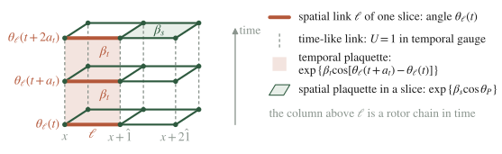
Figure 1. The anisotropic lattice in temporal gauge: along time, every spatial link is an independent rotor chain (temporal plaquettes, coupling ${\beta }_t$); within each slice the spatial plaquettes (coupling ${\beta }_s$) couple the links.

2.2 The transfer matrix

The Hilbert space of a slice is $\mathcal{H}={⨂}_{\ell }{L}^2(S^1,d{\theta }_{\ell }/2\pi )$, with position states normalized by ${\prod }_{\ell }\int \frac{d{\theta }_{\ell }}{2\pi }|\theta ⟩⟨\theta |=1$, so that the Haar measure of the path integral is the resolution of the identity. Splitting each spatial-plaquette weight symmetrically between the two adjacent time steps, $Z=\mathrm{Tr}{T}^{N_t}$ with

$$T=V^{1/2}{T}_E{V}^{1/2},V=\exp [-{\beta }_s\sum _P(1-\cos {\hat{\theta }}_P\left)\right],⟨{\theta }^{\prime }|T_E|\theta ⟩=\prod _{\ell }{e}^{-{\beta }_t[1-\cos ({\theta }_{\ell }^{\prime }-{\theta }_{\ell })]},$$

where $V$ is diagonal in the angles and $T_E$ is a product of Week 1’s rotor-chain kernels, one per link. That kernel is diagonal on the characters: with $\varphi ={\theta }^{\prime }-\theta$,

$${\int }_{-\pi }^{\pi }\frac{d\theta }{2\pi }{e}^{-{\beta }_t[1-\cos ({\theta }^{\prime }-\theta )]}{e}^{in\theta }=e^{in{\theta }^{\prime }}{e}^{-{\beta }_t}{\int }_{-\pi }^{\pi }\frac{d\varphi }{2\pi }{e}^{{\beta }_t\cos \varphi }{e}^{-in\varphi }=e^{-{\beta }_t}{I}_n({\beta }_t)e^{in{\theta }^{\prime }},$$

the Fourier–Bessel coefficient of Week 1 §5.1. Introducing on each link the operator ${\hat{E}}_{\ell }=-i\partial /\partial {\theta }_{\ell }$, with eigenvalue $n$ on $e^{in{\theta }_{\ell }}$,

$$T_E=\prod _{\ell }{e}^{-{\beta }_t}{I}_{{\hat{E}}_{\ell }}({\beta }_t)(I_{-n}=I_n).$$

2.3 The limit $a_t\to 0$ and the Hamiltonian

As $a_t\to 0$ the temporal coupling ${\beta }_t=1/(g^2{a}_t)$ diverges and the Bessel functions are needed at large argument. From the saddle-point expansion of Week 1 §5.2, $I_n(\beta )=\frac{e^{\beta }}{\sqrt{2\pi \beta }}(1-\frac{4n^2-1}{8\beta }+O({\beta }^{-2}))$,

$$\frac{I_n({\beta }_t)}{I_0({\beta }_t)}=1-\frac{n^2}{2{\beta }_t}+O({\beta }_t^{-2})=\exp [-a_t\frac{g^2}{2}{n}^2+O(a_t^2)],$$

while the spatial factor is exactly $V=\exp [-a_t\frac{1}{g^2}{\sum }_P(1-\cos {\hat{\theta }}_P)]$. The symmetric product of three exponentials differs from the exponential of the sum by $O(a_t^3)$, so

$$T=[e^{-{\beta }_t}{I}_0({\beta }_t){]}^{N_{\ell }}{e}^{-a_{t}H+O(a_t^2)},$$

where, dropping the constant $N_P/g^2$,

$$\boxed{H=\frac{g^2}{2}\sum _{\ell }{E}_{\ell }^2-\frac{1}{g^2}\sum _P\cos {\theta }_P=\frac{g^2}{2}\sum _{\ell }{E}_{\ell }^2-\frac{1}{2g^2}\sum _P(U_P+U_P^{†}),E_{\ell }\in \mathbb{Z},}$$

with $U_P=e^{i{\theta }_P}$ the ordered product of the link variables $U_{\ell }=e^{i{\theta }_{\ell }}$ around $P$. This is Kogut’s eq. (6.66) and conventions §4; the physical Hamiltonian is $H/a_s$. The electric term comes from the temporal plaquettes, the magnetic term from the spatial ones, and the coefficient of $\cos {\theta }_P$ is $1/g^2$ because the spatial weight enters the transfer matrix once per time step, with ${\beta }_s=a_t/g^2$.

Two checks. With the Villain weight on the temporal plaquettes the electric factor is exact: its character coefficients are $(2\pi {\beta }_t{)}^{-1/2}{e}^{-n^2/2{\beta }_t}=(2\pi {\beta }_t{)}^{-1/2}{e}^{-a_t{g}^2{n}^2/2}$ (Week 1 §6.2), which is the Euclidean propagator of a particle on a ring of moment of inertia $1/g^2$ over the time $a_t$ (Week 1 §6.1). Each link is literally a quantum rotor with energies $g^2{n}^2/2$. And numerically, the transfer matrix of the one-plaquette system of §6 built with the Wilson weights has a $-\frac{1}{a_t}\ln$-spectrum that converges linearly in $a_t$ to that of $H$ (gaps within 0.2% at $a_t=0.002$, $g=1.3$).

2.4 The photon speed

Keep two independent couplings, ${\beta }_t=1/(g_t^2{a}_t)$ and ${\beta }_s=a_t/g_s^2$. The same steps give $H=\frac{g_t^2}{2}\sum E^2-\frac{1}{g_s^2}\sum \cos {\theta }_P$. At weak coupling the angles are small, $\cos {\theta }_P\simeq 1-\frac{1}{2}{\theta }_P^2$, and the commutator $[{\theta }_{\ell },E_{{\ell }^{\prime }}]=i{\delta }_{\ell {\ell }^{\prime }}$ holds for such fluctuations (fine print F2). The Heisenberg equations of $H\simeq \frac{g_t^2}{2}\Vert E{\Vert }^2+\frac{1}{2g_s^2}\Vert d\theta {\Vert }^2$ are

$${\dot{\theta }}_{\ell }=i[H,{\theta }_{\ell }]=g_t^2{E}_{\ell },{\dot{E}}_{\ell }=i[H,E_{\ell }]=-\frac{1}{g_s^2}(\delta d\theta {)}_{\ell }⟹\ddot{\theta }=-\frac{g_t^2}{g_s^2}\delta d\theta .$$

On transverse modes, $\delta \theta =0$, the operator $\delta d$ equals the Laplacian $\Delta =\delta d+d\delta$ of conventions §2, with eigenvalue ${\hat{k}}^2={\sum }_{i}4{\sin }^2(k_i/2)=k^2+O(k^4)$ on plane waves. Therefore $\omega =(g_t/g_s)\hat{k}$, and the photon speed is $c=g_t/g_s$. Unit speed requires $g_t=g_s$, the relation that the continuum matching of §2.1 imposed, now obtained from the Lorentz invariance of the spectrum alone. The longitudinal modes $\theta =d\lambda$ have $\omega =0$: they are gauge directions, removed by the Gauss law of §4. We checked on $8^2$ and $6^3$ spatial tori that the harmonic Hamiltonian with the coefficients of the box has $\omega /\hat{k}=1.000000$ at the smallest momentum, and that doubling the magnetic term gives $1.414214$.

Physical picture. A simulation of the box would see, at weak coupling, massless photons moving at speed 1 in lattice units; with the magnetic term doubled, $-\frac{1}{g^2}\sum (U_P+U_P^{†})=-\frac{2}{g^2}\sum \cos {\theta }_P$, it would see them moving at $\sqrt{2}$, a theory whose electric and magnetic energies disagree about the speed of light. The mechanism of the correct normalization is the time step: the spatial plaquette weight is paid once per slice, the temporal one is a rotor propagator, and their ratio fixes $c$. The statement is exact at tree level; beyond it the two couplings renormalize differently (F3).

3. The link Hilbert space

3.1 $U(1)$: Fourier series is Peter–Weyl [Proved.]

For $G=U(1)$ the space $L^2(U(1),d\theta /2\pi )$ has the orthonormal basis of characters, $⟨\theta |n⟩=e^{in\theta }$, $n\in \mathbb{Z}$: one state per irreducible representation, which is the Peter–Weyl theorem for the circle. The link operator $\hat{U}$ multiplies by $e^{i\theta }$, so $\hat{U}|n⟩=|n+1⟩$, and $\hat{E}=-i{\partial }_{\theta }$ has $\hat{E}|n⟩=n|n⟩$. For any smooth periodic ψ,

$$[\hat{E},\hat{U}]\psi =-i{\partial }_{\theta }\left(e^{i\theta }\psi \right)+i{e}^{i\theta }{\partial }_{\theta }\psi =e^{i\theta }\psi ,$$

that is, $[E,U]=U$ and $[E,U^{†}]=-U^{†}$; differentiating in α shows $e^{i\alpha E}U{e}^{-i\alpha E}=e^{i\alpha }U$, so $E$ generates rotations of the link, and $U$ raises the electric flux by one unit. The spectrum of $E$ is $\mathbb{Z}$ because the eigenfunctions $e^{ik\theta }$ of $-i{\partial }_{\theta }$ are single-valued on the circle only for integer $k$: compactness of the link variable quantizes the electric flux, in units of $g$ in physical normalization (Kogut RMP 51 §VI.C). The electric energy of a link, $\frac{g^2}{2}{n}^2$, is $\frac{g^2}{2}$ times the quadratic Casimir $n^2$ of the charge-$n$ representation.

3.2 $SU(2)$: left and right generators, and $E^2$ as the Casimir [Proved.]

For $G=SU(2)$ the Peter–Weyl theorem decomposes $L^2(SU(2),dU)={⨁}_{j\in \frac{1}{2}\mathbb{N}}{V}_j\otimes V_j^{\ast }$, with orthonormal basis $\sqrt{2j+1}{D}_{mn}^j(U)$. The group acts on functions by right and left translations, $(R_h\psi )(U)=\psi (Uh)$ and $(L_h\psi )(U)=\psi (h^{-1}U)$, and on the matrix of multiplication operators by $R_h\hat{U}{R}_h^{-1}=\hat{U}h$ and $L_h\hat{U}{L}_h^{-1}=h^{-1}\hat{U}$. Writing $R_h=e^{i{\alpha }^a{E}_R^a}$ and $L_h=e^{i{\alpha }^a{E}_L^a}$ for $h=e^{i{\alpha }^a{T}^a}$, $T^a={\sigma }^a/2$, the first-order terms give

$$[E_R^a,\hat{U}]=\hat{U}{T}^a,[E_L^a,\hat{U}]=-T^a\hat{U},$$

the non-abelian form of $[E,U]=U$ (for $U(1)$, $E_R=E$ and $E_L=-E$). The Jacobi identity, $[[E_R^a,E_R^b],\hat{U}]=\hat{U}[T^a,T^b]$ and $[[E_L^a,E_L^b],\hat{U}]=-[T^a,T^b]\hat{U}$, shows that both sets obey $[E^a,E^b]=i{ϵ}^{abc}{E}^c$, and left and right translations commute, $[E_L^a,E_R^b]=0$. On a Peter–Weyl block,

$$(R_h{D}_{mn}^j)(U)=\sum _k{D}_{mk}^j(U)D_{kn}^j(h),(L_h{D}_{mn}^j)(U)=\sum _k{D}_{mk}^j(h^{-1})D_{kn}^j(U):$$

right translations act on the second index in the spin-$j$ representation and left translations on the first in its contragredient, which for $SU(2)$ is equivalent. Therefore

$$E_L^a{E}_L^a=E_R^a{E}_R^a=j(j+1)\text{on }{V}_j\otimes V_j^{\ast },$$

and the electric energy of a link in the block $j$ is $\frac{g^2}{2}j(j+1)$, the energy of a spherical top of moment of inertia $1/g^2$, which is Kogut and Susskind’s picture. On class functions this is a statement about the Laplacian of the group manifold, the unit three-sphere: with $U=e^{i\psi \hat{n}\cdot \vec{\sigma }}$ the characters are ${\chi }_j=\sin ((2j+1)\psi )/\sin \psi$, and writing $\chi =u/\sin \psi$ turns the radial Laplacian into $\frac{1}{{\sin }^2\psi }{\partial }_{\psi }({\sin }^2\psi {\partial }_{\psi }\chi )=(u^{\prime \prime }+u)/\sin \psi$, so that

$${\nabla }_{S^3}^2{\chi }_j=-[(2j+1{)}^2-1]{\chi }_j=-4j(j+1){\chi }_j,E^a{E}^a=-\frac{1}{4}{\nabla }_{S^3}^2.$$

The electric term is the kinetic energy of a free particle on the group.

3.3 The $SU(N)$ Hamiltonian [Computed for $SU(2)$; Sketched for $SU(N)$.]

The $SU(N)$ Wilson action with $\beta =2N/g^2$ (conventions §4), made anisotropic with ${\beta }_t=2N/(g^2{a}_t)$ and ${\beta }_s=2N{a}_t/g^2$, has the temporal kernel $e^{\frac{{\beta }_t}{N}\mathrm{Re}\mathrm{tr}(U^{\prime }{U}^{†}-1)}$ per link. It is a class function of $U^{\prime }{U}^{-1}$, so by Peter–Weyl and Schur’s lemma the convolution acts on the block $r$ as the number $a_r/d_r=a_0{\tilde{c}}_r({\beta }_t)$, in the notation of the character expansion of conventions §4. For $SU(2)$, with the Haar measure $\frac{2}{\pi }{\sin }^2\psi d\psi$ on class functions and $\mathrm{tr}U=2\cos \psi$,

$$a_j=\frac{2}{\pi }{\int }_0^{\pi }\sin \psi \sin ((2j+1)\psi )e^{\beta \cos \psi }d\psi =I_{2j}(\beta )-I_{2j+2}(\beta )=\frac{2(2j+1)}{\beta }{I}_{2j+1}(\beta ),{\tilde{c}}_j=\frac{I_{2j+1}(\beta )}{I_1(\beta )},$$

where we used $\sin \psi \sin k\psi =\frac{1}{2}[\cos (k-1)\psi -\cos (k+1)\psi ]$, the integral representation of $I_m$ and the recurrence $I_{\nu -1}-I_{\nu +1}=\frac{2\nu }{x}{I}_{\nu }$; at $j=\frac{1}{2}$ this is the $I_2/I_1$ of conventions §4, and we confirmed it by direct Haar integration. At large ${\beta }_t=4/(g^2{a}_t)$ the Bessel expansion gives ${\tilde{c}}_j=1-\frac{(2j+1{)}^2-1}{2{\beta }_t}+O({\beta }_t^{-2})=\exp [-a_t\frac{g^2}{2}j(j+1)+O(a_t^2)]$, which is the Casimir of §3.2. The spatial weight is $\exp [-\frac{a_t}{g^2}{\sum }_P(2N-\mathrm{tr}{U}_P-\mathrm{tr}{U}_P^{†})]$. Thus

$$\boxed{H_{SU(N)}=\frac{g^2}{2}\sum _{\ell }{E}_{\ell }^a{E}_{\ell }^a-\frac{1}{g^2}\sum _P(\mathrm{tr}{U}_P+\mathrm{tr}{U}_P^{†}),}$$

as in conventions §4; for general $N$ the statement ${\tilde{c}}_r({\beta }_t)\to e^{-a_t{g}^2{C}_2(r)/2}$ follows from the Gaussian (heat-kernel) form of the kernel near $U^{\prime }=U$, a step we sketch and do not carry out. The $U(1)$ box of §2.3 and this one use different coupling conventions, $\beta =1/e^2$ against $\beta =2N/g^2$; reading the $SU(N)$ formula at $N=1$ together with the $U(1)$ electric term is the error that produces the doubled magnetic term of the instructor checkpoint.

4. The Gauss law

4.1 Time-independent gauge transformations and $[G_x,H]=0$ [Computed.]

Temporal gauge leaves the time-independent gauge transformations $\theta \to \theta +d\lambda$ (conventions §4). On a slice they are implemented by

$$\mathcal{G}(\lambda )=\exp (i\sum _x{\lambda }_x(\delta E{)}_x)=\exp (i⟨d\lambda ,E⟩),(\delta E{)}_x=\sum _{\mu }[E_{\mu }(x-\hat{\mu })-E_{\mu }(x)],$$

where the second form is the adjointness $⟨\lambda ,\delta E⟩=⟨d\lambda ,E⟩$ of conventions §2, and $(\delta E{)}_x$ is the inflow minus the outflow of electric flux at $x$. Since $e^{i\alpha E}U{e}^{-i\alpha E}=e^{i\alpha }U$ link by link, $\mathcal{G}(\lambda )U_{\ell }\mathcal{G}(\lambda {)}^{-1}=e^{i(d\lambda {)}_{\ell }}{U}_{\ell }$. The electric term commutes with every $(\delta E{)}_x$. For the magnetic term, write $[E_{\ell },U_P]=[\partial P:\ell ]U_P$, with the incidence number $+1$, $-1$ or $0$ according to whether $U_P$ contains $U_{\ell }$, $U_{\ell }^{†}$ or neither, and $(\delta E{)}_x={\sum }_{\ell }[\partial \ell :x]E_{\ell }$. Then

$$[(\delta E{)}_x,U_P]=\sum _{\ell }[\partial \ell :x][\partial P:\ell ]U_P=[\partial \partial P:x]U_P=0:$$

gauge invariance of the magnetic term is ${\partial }^2=0$. Therefore $[(\delta E{)}_x,H]=0$ for every $x$, and the eigenvalues of the $(\delta E{)}_x$ are conserved.

For $SU(N)$, with $U_{\ell }\to {\Lambda }_x^{†}{U}_{\ell }{\Lambda }_{x+\hat{\mu }}$ and $\Lambda =e^{i{\lambda }^a{T}^a}$ (the non-abelian form of $a\to a+d\lambda$), the generator at $x$ is $G_x^a={\sum }_{\ell \text{into}x}{E}_R^a(\ell )+{\sum }_{\ell \text{out of}x}{E}_L^a(\ell )$, which by §3.2 reduces to $(\delta E{)}_x$ for $U(1)$; it commutes with $\mathrm{tr}{U}_P$ because the gauge factors cancel pairwise at each corner of the trace.

4.2 The constraint and the physical projector [Computed.]

Because $[(\delta E{)}_x,H]=0$, the Hilbert space ${⨂}_{\ell }{L}^2(U(1))$ splits into sectors labelled by the integers $(\delta E{)}_x$, and no evolution connects them. A physical state with static charges $q_x$ obeys the Gauss law of conventions §4,

$$(\mathrm{div}E{)}_x|\psi ⟩=\sum _{\mu }[E_{\mu }(x)-E_{\mu }(x-\hat{\mu })]|\psi ⟩=q_x|\psi ⟩,\text{i.e.}\delta E=-q,$$

and the projector onto that sector is, by the Kronecker identity of conventions §3,

$$P_q=\prod _x{\int }_{-\pi }^{\pi }\frac{d{\lambda }_x}{2\pi }{e}^{i{\lambda }_x[(\delta E{)}_x+q_x]},$$

which on an electric-basis state $|E⟩$ gives ${\prod }_x{\delta }_{(\delta E{)}_x,-q_x}$. For $SU(N)$ the constraint reads $(G_x^a+Q_x^a)|\psi ⟩=0$, with $Q_x^a$ the color generators of the static charge at $x$. Without charges the physical states are superpositions of divergence-free integer fluxes, $E\in C^1(\Lambda ,\mathbb{Z})$ with $\delta E=0$: closed electric strings. An open Wilson line ${\prod }_{\ell \in \gamma }{U}_{\ell }$ along a path γ from $x$ to $y$ raises $E$ by one unit on every link of γ in its direction, so it creates $q_x=+1$ and $q_y=-1$: flux lines begin on positive charges.

4.3 Where the constraint comes from: the time-like links [Computed.]

Undo the temporal gauge on one time slice and keep ${\lambda }_x\equiv {\theta }_0(x,t)$ there. The temporal plaquette becomes ${\theta }_{\ell }(t+a_t)-{\theta }_{\ell }(t)-(d\lambda {)}_{\ell }$, so the link kernel is $⟨{\theta }^{\prime }|T_E|\theta +d\lambda ⟩$. Since $\mathcal{G}(\lambda )$ acts on wavefunctions as $\psi (\theta )\mapsto \psi (\theta +d\lambda )$, we have $|\theta +d\lambda ⟩=\mathcal{G}(-\lambda )|\theta ⟩$, and the Haar integral over the time-like links of that slice gives

$$\prod _x{\int }_{-\pi }^{\pi }\frac{d{\lambda }_x}{2\pi }⟨{\theta }^{\prime }|T_E\mathcal{G}(-\lambda )|\theta ⟩=⟨{\theta }^{\prime }|T_E{P}_0|\theta ⟩,$$

using the invariance of the measure under $\lambda \to -\lambda$. The transfer matrix is $T=V^{1/2}{T}_E{P}_0{V}^{1/2}$ and $Z=\mathrm{Tr}(P_0{T}^{N_t})$; since $P_0$ commutes with $T$ and $P_0^2=P_0$, integrating the time-like links of the other slices adds nothing, which is why temporal gauge could be imposed there. The Gauss law is therefore the constraint that the time-like links impose, as a projector; a temporal Wilson line at $x$, a static charge, inserts $e^{\pm i{\lambda }_x}$ and moves the projector to the sector with a charge at $x$.

Physical picture. The Gauss law says that electric flux lines begin and end on charges and nowhere else, and on the lattice this is exact bookkeeping with integers. What breaks if it is dropped is the identification of the vacuum: $H$ alone has eigenstates in every static-charge sector, and without the projector the “ground state” of a pure gauge theory would be a mixture over backgrounds. Confinement is downstream of the constraint: a charge pair must be joined by flux, and at strong coupling flux cannot spread (§5).

5. Strong coupling: strings, their tension and the glueball

5.1 The unperturbed spectrum [Computed.]

At large $g$ we write $H=H_0+V$ with $H_0=\frac{g^2}{2}{\sum }_{\ell }{E}_{\ell }^2$ and $V=-\frac{1}{2g^2}{\sum }_P(U_P+U_P^{†})$. The eigenstates of $H_0$ are the flux configurations $|E⟩$, $E\in C^1(\Lambda ,\mathbb{Z})$, with energy $\frac{g^2}{2}\Vert E{\Vert }^2$; by $[E_{\ell },U_P]=[\partial P:\ell ]U_P$, the magnetic term moves between them with unit amplitude, $U_P|E⟩=|E+\delta 1_P⟩$, adding the boundary of $P$ as a loop of flux. The vacuum is the unique state $E=0$. For static charges $\pm 1$ at $x$ and $y$, the Gauss law requires an integer flow of one unit from $x$ to $y$, and $\Vert E{\Vert }^2\ge {\sum }_{\ell }|E_{\ell }|\ge |x-y{|}_1$, with equality only for a unit flux along a shortest lattice path. For charges on a lattice axis at distance $R$ that path is unique (Figure 2a), and

$$V(R)=\frac{g^2}{2}R,\sigma =\frac{g^2}{2}.$$

For $SU(N)$ the string carries the fundamental representation on every link, $E^a{E}^a=C_2(F)$, and $\sigma =\frac{g^2}{2}{C}_2(F)=\frac{g^2}{2}\frac{N^2-1}{2N}$, equal to $\frac{3g^2}{8}$ for $SU(2)$ (conventions §4). Off-axis separations have many shortest paths, a point taken up in F4.

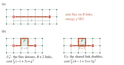
Figure 2. (a) The strong-coupling string between static charges ±1: one unit of electric flux on the straight path. (b) The magnetic term acting on a plaquette that shares one link with the string: one orientation makes the flux detour (cost g²), the other doubles the shared link (cost 3g²).

5.2 The tension at second order [Controlled to $O(g^{-6})$.]

The first-order corrections vanish, since $V$ changes the flux. At second order, $E^{(2)}=-{\sum }_m|⟨m|V|s⟩{|}^2/(E_m-E_s)$ with $|⟨m|V|s⟩|=1/2g^2$. In the vacuum every plaquette offers two moves, each creating a unit loop of energy $2g^2$:

$$E_{\mathrm{vac}}^{(2)}=-N_P\cdot 2\cdot \frac{(1/2g^2{)}^2}{2g^2}=-\frac{N_P}{4g^6}.$$

For the straight string, a plaquette that shares no link with it contributes exactly as in the vacuum; this includes the plaquettes that touch the string only at a site, so the ends add no constant at this order. Each string link lies on $2(D-1)$ plaquettes, and each of these shares only that link with the string (Figure 2b): the move that cancels the shared link costs $\frac{g^2}{2}(-1+3)=g^2$, the one that doubles it costs $\frac{g^2}{2}(4-1+3)=3g^2$, against $2g^2$ twice in the vacuum. Per such plaquette the change is

$$-\frac{1}{4g^4}(\frac{1}{g^2}+\frac{1}{3g^2}-\frac{2}{2g^2})=-\frac{1}{12g^6},\text{so}\boxed{\sigma =\frac{g^2}{2}-\frac{D-1}{6g^6}+O(g^{-14}),}$$

that is, $\frac{g^2}{2}-\frac{1}{6g^6}$ in $2+1$ dimensions and $\frac{g^2}{2}-\frac{1}{3g^6}$ in $3+1$. We checked the counting by enumerating all second-order processes on periodic lattices in $D=2$ and $3$, and the value by exact diagonalization in $2+1$ dimensions (the height variables of Problem 4⋆ on a $2\times 5$ strip of plaquettes): $V(R)-V(R-1)=4.49977136$ at $g=3$, against $4.499771376$. The fluctuations that lower the tension are the detours of Figure 2b, the first transverse vibrations of the string; the energy stays linear in $R$.

5.3 The Euclidean face of the same number [Computed.]

Week 6 found, at leading order of the isotropic strong-coupling expansion, $\sigma =-\ln {\tilde{c}}_1(\beta )=-\ln [I_1(\beta )/I_0(\beta )]$, which at large $g$ and $\beta =1/g^2$ is $\ln (2g^2)$. It is tempting to identify this with $g^2/2$ “up to $\beta \leftrightarrow 1/g^2$”, but $\ln (2g^2)$ and $g^2/2$ are different functions, and no change of variables relates them. The relation is anisotropic. Drop the spatial plaquettes (${\beta }_s\to 0$): in temporal gauge every spatial link is then an independent rotor chain (Figure 1), and a time-like $R\times T$ Wilson loop reduces to its two spatial sides, so that by Week 1 §5.2

$$⟨W(R\times T)⟩=\prod _{\ell \in \gamma }⟨e^{i{\theta }_{\ell }(0)}{e}^{-i{\theta }_{\ell }(T)}⟩=[\frac{I_1({\beta }_t)}{I_0({\beta }_t)}{]}^{RT/a_t},\sigma (a_t)=-\frac{1}{a_t}\ln \frac{I_1({\beta }_t)}{I_0({\beta }_t)}{|}_{{\beta }_t=1/g^2{a}_t}.$$

At $a_t=1$ this is Week 6’s leading-order tension (the spatial plaquettes do not enter the minimal tiling of a time-like loop at that order), and as $a_t\to 0$ the next term of the Bessel expansion, $I_1/I_0=1-\frac{1}{2{\beta }_t}-\frac{1}{8{\beta }_t^2}+\dots$, that is $-\ln (I_1/I_0)=\frac{1}{2{\beta }_t}+\frac{1}{4{\beta }_t^2}+\dots$ with ${\beta }_t=1/g^2{a}_t$, gives $\sigma (a_t)=-\ln [I_1/I_0]({\beta }_t)/a_t=\frac{g^2}{2}+\frac{g^4{a}_t}{4}+O(a_t^2)$, which we confirmed numerically ($0.845715$ at $g=1.3$ and $a_t=10^{-3}$, against $0.845714$ from the two terms). The two tensions are values of one function at two anisotropies. The Hamiltonian strong-coupling regime has ${\beta }_t\to \infty$ and ${\beta }_s\to 0$: its temporal plaquettes are at weak coupling.

5.4 The glueball: degenerate perturbation theory [Controlled to $O(g^{-6})$; computed in $2+1$ dimensions.]

The lightest excitation of the vacuum sector is a unit loop around one plaquette, $|P,s⟩$ with orientation $s=\pm 1$ and energy $4\cdot \frac{g^2}{2}=2g^2$, the smallest closed string. The level is $2N_P$-fold degenerate. Acting on $|P,s⟩$, the magnetic term reaches only the states of the table,

state reached from $|P,s⟩$ by one plaquette move	energy
vacuum (loop removed)	$0$
loop doubled	$8g^2$
second loop on a plaquette $P^{\prime }$ sharing a link, shared link cancelled	$3g^2$
second loop on a plaquette $P^{\prime }$ sharing a link, shared link doubled	$5g^2$
second loop on a plaquette sharing no link	$4g^2$

none of which is degenerate with $2g^2$. Therefore $⟨P^{\prime },s^{\prime }|V|P,s⟩=0$ throughout the manifold: there is no first-order hopping, in any dimension, and the degeneracy survives first order. The effective Hamiltonian starts at second order, $H_{\mathrm{eff}}=PV\frac{Q}{2g^2-H_0}VP$ with $P$ the projector on the manifold and $Q=1-P$, and each process contributes $\frac{1}{4g^4}(2g^2-E_m{)}^{-1}$. Its entries in $2+1$ dimensions are as follows.

• Diagonal. Summing the rows of the table, with four edge-neighbours of $P$ and $N_P-5$ plaquettes sharing no link, each in two orientations,

$$\frac{1}{4g^4}[\frac{1}{2g^2}-\frac{1}{6g^2}+4(-\frac{1}{g^2}-\frac{1}{3g^2})+2(N_P-5)(-\frac{1}{2g^2}\left)\right]=-\frac{N_P}{4g^6}=E_{\mathrm{vac}}^{(2)}:$$

the on-site energy is unshifted relative to the vacuum. (In $D$ dimensions the same count, with $4(2D-3)$ plaquettes sharing a link with $P$, gives the shift $\frac{4-2D}{3g^6}$, that is $-\frac{2}{3g^6}$ in $3+1$ dimensions.)

• Orientation flip on the same plaquette, through the vacuum: $⟨P,-s|H_{\mathrm{eff}}|P,s⟩=+\frac{1}{8g^6}$.
• Hopping to a plaquette $P^{\prime }$ sharing a link, along the two orders (remove $P$ then add $P^{\prime }$, or the reverse): $\frac{1}{4g^4}(\frac{1}{2g^2}-\frac{1}{g^2})=-\frac{1}{8g^6}$ when the shared link cancels in the intermediate state (the same orientation, for coplanar neighbours), and $\frac{1}{4g^4}(\frac{1}{2g^2}-\frac{1}{3g^2})=+\frac{1}{24g^6}$ when it doubles.
• Plaquettes sharing no link: $\frac{1}{4g^4}(\frac{1}{2g^2}-\frac{1}{2g^2})=0$. The two orders cancel, which keeps the hopping local.

Charge conjugation $E\to -E$ exchanges $s=\pm 1$. In the combinations $C=\pm$, the on-site energy is $\pm \frac{1}{8g^6}$ and the hopping $t_{\pm }=-\frac{1}{8g^6}\pm \frac{1}{24g^6}$, so $t_{+}=-\frac{1}{12g^6}$, $t_{-}=-\frac{1}{6g^6}$, and the bands on the square lattice are $m_{\pm }(k)=2g^2\pm \frac{1}{8g^6}+2t_{\pm }(\cos k_1+\cos k_2)$. Their minima at $k=0$ are

$$\boxed{m_{-}=2g^2-\frac{19}{24g^6},m_{+}=2g^2-\frac{5}{24g^6}(2+1\text{dimensions}).}$$

The $C$-odd state, created from the vacuum by $\sin {\theta }_P$, the lattice magnetic field, is the lighter; it carries the quantum numbers of the photon, which at weak coupling becomes the massive photon of compact QED${}_3$ (Week 9). On the $3\times 3$ torus these bands predict eighteen levels above the vacuum, $2g^2+\{-19,-7^{(4)},-5,1^{(4)},5^{(4)},7^{(4)}\}/24g^6$, and exact diagonalization reproduces all of them ($g=3.5$, heights truncated at $|h|\le 2$). The glueball therefore moves only when the magnetic term acts twice, as Kogut and Susskind observed (§VII of their paper), and its mass gap $2g^2+O(g^{-6})$ is the strong-coupling statement that the pure gauge theory is gapped.

6. The one-plaquette universe [Computed.]

6.1 Reduction by the Gauss law

Consider a single plaquette: four sites, four links, $\partial P={\ell }_1+{\ell }_2-{\ell }_3-{\ell }_4$ (bottom, right, top, left). The Gauss law $\delta E=0$ at the four corners reads $-(E_1+E_4)=0$, $E_1-E_2=0$, $E_4-E_3=0$ and $E_2+E_3=0$, so $E=n(1,1,-1,-1)=n\delta 1_P$ and ${\sum }_{\ell }{E}_{\ell }^2=4n^2$. The physical space is ${\ell }^2(\mathbb{Z})$ with $U_P|n⟩=|n+1⟩$. Equivalently, a gauge-invariant wavefunction depends on the angles only through $\varphi ={\theta }_P={\theta }_1+{\theta }_2-{\theta }_3-{\theta }_4$, and ${\sum }_{\ell }(-{\partial }_{{\theta }_{\ell }}^2)f(\varphi )=-4f^{\prime \prime }(\varphi )$. Either way,

$$\boxed{H_1=2g^2{\hat{n}}^2-\frac{1}{g^2}\cos \varphi ,\hat{n}=-i{\partial }_{\varphi },\psi (\varphi +2\pi )=\psi (\varphi ),}$$

a rotor in a cosine potential. With $\varphi =2z$ it is the Mathieu equation ${\psi }^{\prime \prime }+(a-2q\cos 2z)\psi =0$, where $a=2E/g^2$ and $q=-1/g^4$, restricted to its π-periodic solutions: one parameter, $g^4$, the ratio of the two terms. We checked the reduction against the four-link system with the Gauss law imposed by enumeration.

6.2 Strong coupling [Controlled to $O(g^{-6})$.]

At $g\to \infty$, $E_n=2g^2{n}^2$, with $n=\pm 1$ degenerate. The ground state gets $E_0=-2\cdot \frac{(1/2g^2{)}^2}{2g^2}=-\frac{1}{4g^6}$. On $\{|1⟩,|-1⟩\}$ the second-order effective Hamiltonian has the diagonal $\frac{1}{4g^4}[\frac{1}{2g^2}+\frac{1}{2g^2-8g^2}]=\frac{1}{12g^6}$ (through $n=0$ and $n=\pm 2$) and the off-diagonal $\frac{1}{4g^4}\cdot \frac{1}{2g^2}=\frac{1}{8g^6}$ (through $n=0$), so

$$E_{\sin }=2g^2-\frac{1}{24g^6},E_{\cos }=2g^2+\frac{5}{24g^6},$$

for the $C$-odd and $C$-even combinations. The off-diagonal element is the on-site orientation flip of §5.4. These values match the small-$q$ series of the Mathieu characteristic values $b_2(q)$ and $a_2(q)$, and the exact diagonalization to $10^{-8}$ at $g=3$.

6.3 Weak coupling [Controlled to $O(g^2)$; tunneling Heuristic.]

At small $g$ the wavefunction sits near $\varphi =0$. Expanding $-\frac{1}{g^2}\cos \varphi =-\frac{1}{g^2}+\frac{{\varphi }^2}{2g^2}-\frac{{\varphi }^4}{24g^2}+\dots$ and writing the kinetic term as $p^2/2m$ with $m=1/4g^2$, the oscillator condition $\frac{1}{2}m{\omega }^2=\frac{1}{2g^2}$ gives

$${\omega }^2=\frac{4g^2}{g^2}=4,\omega =2,$$

independent of $g$: it is the photon of §2.4 on the single mode, whose $\delta d$-eigenvalue is $\Vert \delta 1_P{\Vert }^2=4$. The quartic term at first order, with $⟨{\varphi }^4{⟩}_n=\frac{3}{4m^2{\omega }^2}(2n^2+2n+1)=3g^4(2n^2+2n+1)$, gives

$$E_n=-\frac{1}{g^2}+(2n+1)-\frac{g^2}{8}(2n^2+2n+1)+O(g^4),E_1-E_0=2-\frac{g^2}{2}+O(g^4),$$

confirmed numerically (gap $1.996795$ at $g=0.08$, against $1.996800$). Beyond all orders the angle can tunnel through $2\pi$: the WKB action is ${\int }_0^{2\pi }\sqrt{2m(1-\cos \varphi )/g^2}d\varphi =\frac{1}{g^2}{\int }_0^{2\pi }|\sin \frac{\varphi }{2}|d\varphi =\frac{4}{g^2}$, so the energies depend on a twist of the boundary condition only through $e^{-4/g^2}$ (Problem 8⋆⋆). The tunneling event changes the magnetic flux through the plaquette by $2\pi$; it is the one-plaquette ancestor of the monopole instanton of Week 9 and Week 10, which breaks explicitly the magnetic symmetry, a 0-form symmetry in $2+1$ dimensions (conventions §6).

Figure 3 shows the crossover between the two descriptions.

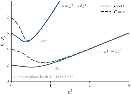
Figure 3. The four lowest excitation energies $E-E_0$ of the one-plaquette universe (computed by exact diagonalization of $H_1$, §6.1): equally spaced oscillator levels with ω = 2 at weak coupling, electric-flux levels 2g²n² at strong coupling, and a smooth crossover near g² ≈ 0.5–1.

7. The ${\mathbb{Z}}_2$ theory and its dual Ising model

7.1 The ${\mathbb{Z}}_2$ Kogut–Susskind Hamiltonian [Computed.]

Wegner’s action made anisotropic, $S=-{\beta }_t{\sum }_{P_t}{\sigma }_P-{\beta }_s{\sum }_{P_s}{\sigma }_P$, becomes in temporal gauge one Ising chain in time per spatial link. With $s=\pm 1$ the eigenvalue of ${\sigma }^z$, the link kernel is

$$⟨s^{\prime }|T_E|s⟩=e^{{\beta }_t{s}^{\prime }s}=e^{{\beta }_t}{\delta }_{s^{\prime }s}+e^{-{\beta }_t}{\delta }_{s^{\prime },-s},\text{i.e.}{T}_E=e^{{\beta }_t}(1+e^{-2{\beta }_t}{\sigma }^x)=\frac{e^{{\beta }_t}}{\cosh {\beta }_t^{\ast }}{e}^{{\beta }_t^{\ast }{\sigma }^x},\tanh {\beta }_t^{\ast }=e^{-2{\beta }_t},$$

where ${\beta }_t^{\ast }$ is the Kramers–Wannier dual coupling of Week 4 §3.3. The limit is taken with $e^{-2{\beta }_t}=a_t\Gamma$ and ${\beta }_s=a_{t}K$, so that $T\propto e^{-a_{t}H+O(a_t^2)}$ with

$$\boxed{H=-\Gamma \sum _{\ell }{\sigma }_{\ell }^x-K\sum _P{B}_P,B_P=\prod _{\ell \in \partial P}{\sigma }_{\ell }^z,\prod _{\ell \ni v}{\sigma }_{\ell }^x=(-1{)}^{q_v},}$$

the normalization of conventions §4, with Γ and $K$ energies; only $K/\Gamma$ matters for the phases. The dictionary with §3 is the ${\mathbb{Z}}_2$ Peter–Weyl theorem. The two characters of a link are ${\chi }_0(s)=1$ and ${\chi }_1(s)=s$, which are the ${\sigma }^x$ eigenstates with eigenvalues $+1$ and $-1$. Thus ${\sigma }^x=(-1{)}^E$ with $E\in \{0,1\}$ is the electric field, and ${\sigma }^z=U$, multiplication by $s$, exchanges ${\chi }_0$ and ${\chi }_1$: it flips the electric flux. The Gauss law is the mod-2 form of §4.2, in which the orientation signs drop out. A link carrying flux costs $2\Gamma$, so the strong-coupling tension is $2\Gamma$.

7.2 The two-level universe [Computed.]

On one plaquette the Gauss law ${\sigma }_{\ell }^x{\sigma }_{{\ell }^{\prime }}^x=1$ at each corner forces all four ${\sigma }^x$ to be equal: of sixteen states two are physical, $|+⟩$ (no flux) and $|-⟩$ (one ${\mathbb{Z}}_2$ flux loop), and $B_P$ exchanges them. So

$$H=\left(\begin{array}{cc}-4\Gamma & -K\\ -K& 4\Gamma \end{array}\right),E_{\pm }=\pm \sqrt{16{\Gamma }^2+K^2},\Delta =2\sqrt{16{\Gamma }^2+K^2}.$$

The gap never closes. The ground state $\cos \alpha |+⟩+\sin \alpha |-⟩$ with $\tan 2\alpha =K/4\Gamma$ turns from electric ($\alpha =0$) to magnetic ($\alpha =\pi /4$), and the crossover, $\alpha =\pi /8$, sits at $K=4\Gamma$, where the two terms have equal strength. There is no transition and no self-dual point; along the line $K=1/\Gamma$ the gap $2\sqrt{16{\Gamma }^2+{\Gamma }^{-2}}$ has a minimum at $\Gamma =\frac{1}{2}$, which is a crossover.

7.3 Duality to the transverse-field Ising model [Computed.]

On the plane, without charges, place Pauli operators on the dual sites (plaquette centres, Figure 4):

$${\mu }_P^x\equiv B_P,{\mu }_P^z\equiv \prod _{\ell \text{crossed by}{\tilde{\gamma }}_P}{\sigma }_{\ell }^x,$$

where ${\tilde{\gamma }}_P$ is a dual path from $P$ to infinity. Four facts make this a change of variables on the physical space.

1. Both are gauge invariant: they commute with every $A_v={\prod }_{\ell \ni v}{\sigma }_{\ell }^x$.
2. ${\mu }_P^z$ is independent of the path. Two paths differ by a closed dual loop, and the product of ${\sigma }^x$ over the links crossed by a closed dual loop is the product of the $A_v$ over the enclosed sites, which is 1 by the Gauss law. This is the seam argument of Week 4 §4.1, now enforced by a constraint.
3. The Pauli algebra holds. $B_P$ anticommutes with ${\mu }_Q^z$ exactly when $\partial P$ and ${\tilde{\gamma }}_Q$ share an odd number of links; a path through $P$ crosses $\partial P$ twice, so this happens only for $P=Q$.
4. For the two plaquettes $P,P^{\prime }$ that share the link ℓ, choosing ${\tilde{\gamma }}_P=\ell \cup {\tilde{\gamma }}_{P^{\prime }}$ gives ${\mu }_P^z{\mu }_{P^{\prime }}^z={\sigma }_{\ell }^x$.

Therefore, on the physical space,

$$\boxed{H=-\Gamma \sum _{⟨P{P}^{\prime }⟩}{\mu }_P^z{\mu }_{P^{\prime }}^z-K\sum _P{\mu }_P^x,}$$

the transverse-field Ising model on the dual lattice, with Ising coupling Γ and transverse field $K$ (conventions §4; Kogut RMP 51 §V.E; Fradkin and Susskind 1978). The phase map follows at once. For $\Gamma \gg K$ the gauge theory is at strong coupling and confined, and the Ising model is a ferromagnet, $⟨{\mu }^z⟩\ne 0$; for $K\gg \Gamma$ the gauge theory is deconfined and the Ising model is a paramagnet. The Ising order parameter ${\mu }_P^z$ is a string of electric field ending at $P$, which flips $B_P$ there: it creates a ${\mathbb{Z}}_2$ magnetic flux, a vison, and it is a local operator of the dual model. Visons condense in the confined phase, which is Kogut’s eq. (5.69) in his notation. The transition is continuous and in the three-dimensional Ising class, the Hamiltonian face of the Euclidean duality $\tanh \beta =e^{-2K^{\ast }}$ of Week 5, with the same assignment of phases; its location is a single number, the critical point of the square-lattice transverse-field Ising model, $(K/\Gamma {)}_c\approx 3.044$, known from simulations [Stated — refs: Blöte–Deng, Phys. Rev. E 66 (2002) 066110]. Adding ${\mathbb{Z}}_2$ matter on the sites turns this model into the gauge–Higgs system of Week 13, whose Hamiltonian phase diagram is drawn with exactly these variables.

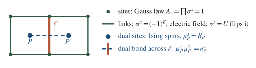
Figure 4. The duality geometry: the Ising spins live on plaquette centres, the magnetic term is their transverse field, and the electric field on a link is the Ising bond across it.

Physical picture. What a simulation of the gauge theory sees as confinement, an area law of $⟨{\prod }_{\ell \in C}{\sigma }_{\ell }^z⟩$, is on the dual side ferromagnetic order of visons, and deconfinement is their disorder; this correspondence is exact (§7.3). The mechanism is the one Week 4 met for Kramers–Wannier: a disorder operator, here ${\mu }^z$, condenses where the order variable cannot. For the research line of the course this is the simplest instance of confinement as the condensation of magnetic defects, the ${\mathbb{Z}}_2$ version of the dual superconductor of Week 11 and of the defect condensation of the julia-toulouse-mechanism, which returns in modern dress in Semester II Week 14 (forward reference, heuristic at this stage).

7.4 On the torus: flux sectors and the missing states [Computed.]

On an $L_1\times L_2$ torus with $N$ sites, $2N$ links and $N$ plaquettes, the $N$ Gauss constraints obey one relation, ${\prod }_v{A}_v=1$, so the physical space has dimension $2^{2N}/2^{N-1}=2^{N+1}$, twice the $2^N$ states of the dual spins. The bookkeeping is exact. First, ${\prod }_P{B}_P=1$ identically (every link lies on two plaquettes), so ${\prod }_P{\mu }_P^x=1$: the dual model lives in its ${\mathbb{Z}}_2$-even sector. Second, the electric fluxes through the two non-contractible dual cycles, $U_i={\prod }_{\ell \in {\tilde{C}}_i}{\sigma }_{\ell }^x$, commute with $H$ and label four sectors. They are the generators of the ${\mathbb{Z}}_2$ electric 1-form symmetry, supported on closed curves of the spatial slice, and they anticommute with the Wilson loops that cross them once, which are the charged objects (conventions §6). The product of ${\mu }^z{\mu }^z$ around a closed dual cycle equals the flux through it, so in the sector where electric flux winds along direction 1 the dual spins are antiperiodic along direction 2, and vice versa. Thus $4\times 2^{N-1}=2^{N+1}$. We checked on the $3\times 3$ torus that the spectra agree sector by sector to $10^{-13}$, and on the $3\times 4$ torus that the pairing of directions is the one just stated. This is the sector structure of Week 4 §3.4, here as a direct sum; in the deconfined phase the four sectors become degenerate, which is the degeneracy of §8.

8. The energetic Gauss law and the toric-code point [Proved.]

The Gauss law can be imposed as an energy instead of a constraint. Consider $H_h=H-h{\sum }_v{A}_v$ with $h>0$, on the full space of link qubits. Since $[A_v,H]=0$, $H_h$ is block diagonal in the eigenvalues of all the $A_v$. In the block with $A_v=1$ for every $v$ it equals $H-hN$; the other blocks are the static-charge sectors of $H$, each charge costing an extra $2h$. So the two formulations coincide exactly on the physical sector, and the energetic one keeps the charged sectors as gapped excitations instead of discarding them. At $\Gamma =0$, where $H=-K{\sum }_P{B}_P$ is the same in every charge sector, the ground state lies in the charge-free block for every $h>0$. Setting $K=h=1$ there,

$$\boxed{H_{\mathrm{TC}}=-\sum _v{A}_v-\sum _P{B}_P,}$$

Kitaev’s toric code (conventions §9): the $\Gamma \to 0$ point of the ${\mathbb{Z}}_2$ Kogut–Susskind Hamiltonian with the magnetic term rescaled and the Gauss law imposed energetically. Adding $-{\sum }_v{A}_v$ at $\Gamma \ne 0$ gives the toric code plus $-\Gamma {\sum }_{\ell }{\sigma }_{\ell }^x$, and no regrouping removes that term, since $A_v$ is the product of the four ${\sigma }^x$ at $v$ while the electric term is their sum. The two sets of terms of $H_{\mathrm{TC}}$ commute, $[A_v,B_P]=0$, because a star and a plaquette share zero or two links; the ground states have $A_v=B_P=1$, and in the electric basis each is an equal-weight superposition of closed ${\mathbb{Z}}_2$ flux loops within one of the four sectors of §7.4, which at $\Gamma =0$ all have the energy $-KN$: four ground states on the torus (checked on $3\times 3$). Switching Γ back on gives the toric code in a field along $x$, which is the pure gauge theory of §7 in each charge sector and has the three-dimensional Ising transition of its dual Ising model (Trebst et al. 2007). The anyons, the $2^{2g}$ degeneracy and the entanglement are Semester II Week 8 (Block 3, Week 8): a Gauss-law violation is the $e$ particle, and a plaquette with $B_P=-1$ is the $m$ particle, the vison of §7.3.

9. Subtleties and fine print

F1 — Temporal gauge and the residual gauge freedom. Setting $U_0=1$ on every time-like link is possible on a lattice open in time. On a periodic one it is possible on all slices but one, because the Polyakov loops ${\prod }_t{U}_0(x,t)$ are gauge invariant; the links of the remaining slice are the λ of §4.3, whose integral is the projector. Temporal gauge leaves the time-independent gauge transformations, generated by $(\delta E{)}_x$, and loses the equation of the time-like link, which must then be imposed on states as the Gauss law.

F2 — Why $E$ is an integer, and why $[\theta ,E]=i$ is only formal. The integer spectrum is the single-valuedness of $e^{ik\theta }$ (§3.1). A canonical pair $(\theta ,E)$ does not exist on the circle: the diagonal matrix element $⟨n|[\hat{\theta },\hat{E}]|n⟩=n⟨n|\hat{\theta }|n⟩-n⟨n|\hat{\theta }|n⟩=0$ contradicts $[\theta ,E]=i$, because multiplication by the discontinuous function θ does not preserve the domain of $\hat{E}$. The consistent algebra is $[E,U]=U$ with $U{U}^{†}=1$. The canonical commutator returns as an approximation for wavefunctions concentrated away from the cut, which is why the weak-coupling frequencies of §§2.4 and 6.3 are right. A non-compact lattice gauge field would have continuous $E$ and no strings.

F3 — Ordering and the uniqueness of the limit. (i) Splitting $V$ symmetrically or not changes $T$ by commutators of order $a_t^2$ and leaves $H$ unchanged. (ii) The Wilson, Villain and heat-kernel temporal weights give the same $H$, the Villain weight with no correction at all (§2.3); the Bessel expansion is not uniform in $n$, so the limit holds on states of bounded electric energy. (iii) For $SU(N)$ the left and right generators of a link differ by parallel transport through it, $E_L=-U{E}_R{U}^{†}$ in matrix notation, and the electric term is their common Casimir, so the lattice Hamiltonian has no ordering ambiguity; ambiguities of this kind enter only through the irrelevant operators ($E^4$ terms, larger loops) that improved Hamiltonians add, and these change no universal quantity. (iv) The equality $g_t=g_s$ that gives $c=1$ is a tree-level statement: quantum corrections renormalize the two couplings differently, so that at finite coupling the ratio must be retuned to keep the renormalized speed of light at one. We do not compute this correction.

F4 — Strong coupling breaks rotations. For a separation off the lattice axes the minimal strings are all the shortest lattice paths, a degenerate multiplet that the magnetic term mixes at first order by moving corners. At leading order $V(R)$ grows with the ${\ell }^1$ length $|R{|}_1$, so the tension along a diagonal is $\sqrt{2}$ times the on-axis one. Rotational invariance can return only where the string roughens, near the continuum limit (Kogut RMP 55 §V.C). Note also that the strong-coupling string of compact $U(1)$ in $3+1$ dimensions is a lattice phase, separated from the weak-coupling Coulomb phase by a transition (Week 11), while in $2+1$ dimensions confinement persists at all couplings (Weeks 9–10).

F5 — Staggered fermions, named and set aside. Kogut and Susskind’s paper opens (§II) with fermions on the spatial lattice, distinguishing even and odd sites, the germ of the staggered fermions of later work (Kogut RMP 55 §§VII.C–E). Dynamical fermions, species doubling and lattice chiral symmetry are outside this course; our charges are static.

F6 — Why the duality is set in $2+1$ dimensions. In $1+1$ dimensions a pure gauge chain has no plaquettes, $H=-\Gamma \sum {\sigma }^x$, and on a ring the Gauss law makes all ${\sigma }^x$ equal: the physical space has two states, the two values of the electric flux, and there is nothing to dualize. A chain version of the gauge–Ising correspondence needs matter (Problem 5⋆, and the gauging of Semester II Week 4). The $2+1$-dimensional statement of §7.3 is the one that Week 5’s three-dimensional duality predicts.

F7 — Global structure of the $U(1)$ theory on a torus. Every link lies on two plaquettes with opposite orientations, so ${\prod }_P{U}_P=1$, and the zero-winding physical states of $2+1$ dimensions are $E=\delta h$ with integer heights $h$ defined up to a global shift. The electric fluxes around the cycles are conserved integers, and the glueball calculation of §5.4 lives in the zero-winding sector.

10. Common misconceptions

• “The Hamiltonian and the Euclidean formulations could disagree about the phases.” It is tempting because their numbers differ: $\sigma =g^2/2$ against $-\ln (I_1/I_0)(\beta )$, and critical couplings that do not coincide. The Hamiltonian is the $a_t\to 0$ end of a one-parameter family of Euclidean lattices with the same symmetries (§2), and along that family the phases and the universality classes do not change: the ${\mathbb{Z}}_2$ theory is three-dimensional Ising in both, through the same assignment of confined to ordered (§7.3 and Week 5). Only non-universal numbers depend on the anisotropy, and §5.3 computes how.
• “The Gauss law is an equation of motion.” In continuum Maxwell theory it is the Euler–Lagrange equation of $A_0$, so the confusion is natural. In the Hamiltonian lattice theory the Heisenberg equations of $H$ do not imply it: $[G_x,H]=0$ only says that $G_x$ is conserved, and the Hilbert space contains every static-charge sector. The Gauss law selects one of them; it enters the transfer matrix as the projector produced by the time-like links (§4.3).
• “The strong-coupling tensions of the two formulations match after $\beta \leftrightarrow 1/g^2$.” They are values of one function at two anisotropies (§5.3). The same care applies to the glueball: its level is degenerate and first-order perturbation theory gives nothing, so it moves at order $1/g^6$ (§5.4).
• “Adding $-{\sum }_v{A}_v$ to the ${\mathbb{Z}}_2$ Kogut–Susskind Hamiltonian gives the toric code.” The electric term $-\Gamma \sum {\sigma }^x$ remains; the toric code is the point $\Gamma =0$ with the energetic Gauss law (§8).

11. Historical note

Kogut and Susskind (received July 1974, published January 1975) presented Wilson’s lattice model as a canonical Hamiltonian theory for $SU(2)$ with fermions, on a spatial lattice with continuous time. Their language was the rigid rotator: each link variable is the orientation of a spherical top, the space-fixed and body-fixed angular momenta generate the gauge transformations at the two ends of the link, and the moment of inertia $a/g^2$ was fixed by matching the classical continuum limit; the derivation from the anisotropic transfer matrix that we followed is the one of Kogut’s reviews (RMP 51 §VI.C; RMP 55 §V.A). They built the gauge-invariant configuration space as strings of non-abelian electric flux ending on quarks, found the energy of a separated pair linear in its distance at strong coupling, computed the corrections in inverse powers of the coupling as fluctuations of the strings, identified the lightest pure-gauge excitation as a four-link box of energy $3g^2/2a$ (Problem 1), and noted that it propagates only when the plaquette term acts twice. Fradkin and Susskind (1978) then worked out the Hamiltonian dualities of the ${\mathbb{Z}}_2$ theories, and Kitaev’s toric code (1997), a quantum error-correcting code built on anyons, is the $\Gamma =0$ point of §8.

12. What to take away

1. The Hamiltonian is a limit. With ${\beta }_t=1/g^2{a}_t$ and ${\beta }_s=a_t/g^2$, the transfer matrix gives $H=\frac{g^2}{2}\sum E^2-\frac{1}{g^2}\sum \cos {\theta }_P$: the electric term is the rotor-chain Bessel ratio, the magnetic term the spatial plaquette weight, and photons move at unit speed. Physically, every link is a quantum rotor.
2. Flux is quantized by compactness. $E\in \mathbb{Z}$ with $[E,U]=U$; for $SU(2)$, $E^a{E}^a=j(j+1)$ is the Casimir of the Peter–Weyl block, the kinetic energy of a particle on the group.
3. The Gauss law is a projector. It comes from the time-like links, $[G_x,H]=0$ is ${\partial }^2=0$, physical states are closed strings, and charges are their ends.
4. Strong coupling confines. $\sigma =\frac{g^2}{2}-\frac{D-1}{6g^6}$ for $U(1)$, and $\frac{g^2}{2}{C}_2(F)$ for $SU(N)$ at leading order; the glueball of mass $2g^2$ is degenerate at first order and hops at order $1/g^6$, with the $C$-odd state lighter in $2+1$ dimensions.
5. One plaquette interpolates. $2g^2{n}^2$ at strong coupling, ω = 2 at weak coupling, a smooth crossover in between; the ${\mathbb{Z}}_2$ gap $2\sqrt{16{\Gamma }^2+K^2}$ never closes.
6. ${\mathbb{Z}}_2$ is dual to Ising. ${\sigma }^x$ is the electric field and ${\sigma }^z$ flips it; the dual transverse-field Ising model is ferromagnetic in the confined phase, the torus sectors are its boundary conditions, and the toric code is the point $\Gamma =0$ with the Gauss law imposed energetically.

13. Looking ahead: Week 8

Week 8 opens with the midterm and then builds the dual variables of abelian lattice gauge theories (Week 8): the Villain gauge action is Poisson-resummed, a dual integer field appears, and the monopoles are localized on the dual lattice. The heights $h$ of Problem 4⋆, with $E=\delta h$, are the Hamiltonian form of that dual integer field in $2+1$ dimensions, and the tunneling of §6.3 is the Hamiltonian form of its monopoles. In three dimensions these are points, and Polyakov’s mechanism follows in Weeks 9–10.

14. Problem set

Problems 1–3 are the classroom core and are solvable from this note; 4⋆, 5⋆ and 6⋆ are self-study consolidation, each with its method indicated; 7⋆⋆ and 8⋆⋆ are research extensions, each stating what is known, what is explored, its sources and what counts as completion.

Core problems (everyone).

1. The $SU(2)$ one-plaquette universe: matrix elements in the electric basis. This extends §6 to the non-abelian group with the tools of §3.2. (a) Show that the gauge-invariant states of one $SU(2)$ plaquette are the class functions of $U_P$, that ${\sum }_{\ell }{E}_{\ell }^a{E}_{\ell }^a{\chi }_j(U_P)=4j(j+1){\chi }_j(U_P)$, and that the magnetic term is $-\frac{2}{g^2}{\chi }_{1/2}(U_P)$. With the Clebsch–Gordan series ${\chi }_{1/2}{\chi }_j={\chi }_{j+1/2}+{\chi }_{j-1/2}$ (and ${\chi }_{1/2}{\chi }_0={\chi }_{1/2}$), write $H$ in the orthonormal character basis. (b) At strong coupling find the ground energy and the gap to second order in $1/g^2$, and compare the leading gap with the energy of a fundamental string of four links (§5.1). (c) At weak coupling use $E^a{E}^a=-\frac{1}{4}{\nabla }_{S^3}^2$ to reduce $H$ near $U_P=1$ to an isotropic oscillator in three dimensions acting on class functions, and find the gap.

2. The two-plaquette universe. This is §§5.4 and 6 on the smallest system with a shared link. (a) For two plaquettes sharing a link (six sites, seven links), both oriented counterclockwise, solve the Gauss law and show that the physical states are $|n_1,n_2⟩$ with $H=\frac{g^2}{2}[3n_1^2+3n_2^2+(n_1-n_2{)}^2]-\frac{1}{g^2}(\cos {\varphi }_1+\cos {\varphi }_2)$. (b) Find the two weak-coupling frequencies and check that they do not depend on $g$. (c) At strong coupling show that the four single-loop states $|\pm 1,0⟩$ and $|0,\pm 1⟩$ are not connected at first order, compute the second-order effective Hamiltonian among them (the amplitudes of §5.4 apply to the off-diagonal entries; recompute the diagonal ones, since this geometry is not the bulk), and find the four levels relative to the ground state. Check them by diagonalizing $H$ numerically in a truncated basis.

3. Charge-2 static sources. This extends §§5.1–5.2 to a doubled charge. (a) Place charges $+2$ and $-2$ on a lattice axis at separation $R$. At leading order compare the doubled string, $2g^{2}R$, with configurations of two unit strings, and find the minimal configurations and their number for $R\ge 2$ in $2+1$ and $3+1$ dimensions. Conclude that ${\sigma }_2=2{\sigma }_1$ at strong coupling, and explain why the charge-2 flux does not stay in one tube. (b) At $R=1$ show that the doubled link is degenerate with the configurations in which one unit of flux detours around an adjacent plaquette, count them, and diagonalize the magnetic term on this manifold at first order to find the ground energy in $2+1$ and $3+1$ dimensions.

Starred problems.

4⋆. Heights: the $U(1)$ theory in $2+1$ dimensions in dual variables. Show that on the plane every charge-free physical configuration is $E=\delta h$ with $h$ a unique integer 2-cochain (a height on every dual site), that $U_P$ raises $h_P$ by one, and that

$$H=\frac{g^2}{2}\sum _{⟨P{P}^{\prime }⟩}(h_P-h_{P^{\prime }}{)}^2-\frac{1}{g^2}\sum _P\cos {\phi }_P,[h_P,e^{i{\phi }_{P^{\prime }}}]={\delta }_{P{P}^{\prime }}{e}^{i{\phi }_P}.$$

Reduce mod 2 to recover §7.3, describe the torus (global shift and winding sectors, F7), and say which object of Week 8 the integer $h$ becomes. (Method: the integer solution of $\delta E=0$ in Week 3 §3, read on the spatial lattice.)

5⋆. The ${\mathbb{Z}}_2$ gauge chain with matter. In $1+1$ dimensions put Ising matter τ on the sites and gauge qubits on the links, with

$$H=-h\sum _i{\tau }_i^x-J\sum _i{\tau }_i^z{\sigma }_{i,i+1}^z{\tau }_{i+1}^z-\Gamma \sum _i{\sigma }_{i,i+1}^x,{\sigma }_{i-1,i}^x{\tau }_i^x{\sigma }_{i,i+1}^x=1.$$

Show that $X_{\ell }={\sigma }_{\ell }^x$ and $Z_{\ell }={\tau }_i^z{\sigma }_{\ell }^z{\tau }_{i+1}^z$ form a gauge-invariant Pauli pair on each link $\ell =(i,i+1)$, count the physical states on a ring, and write $H=-h\sum X_{\ell }{X}_{\ell +1}-J\sum Z_{\ell }-\Gamma \sum X_{\ell }$. Identify the $\Gamma =0$ model with the Kramers–Wannier dual of the matter chain (Week 4 §4.4), and interpret Γ as the tension of the electric string that binds matter charges. (Hint: on the physical space ${\tau }_i^x=X_{i-1,i}{X}_{i,i+1}$; this is the chain version that F6 promises.)

6⋆. The anisotropic tension and the Villain time step. (a) With the next term of the Bessel expansion, $I_{\nu }(z)\simeq \frac{e^z}{\sqrt{2\pi z}}[1-\frac{\mu -1}{8z}+\frac{(\mu -1)(\mu -9)}{2(8z{)}^2}]$ with $\mu =4{\nu }^2$, derive $\sigma (a_t)=\frac{g^2}{2}+\frac{g^4{a}_t}{4}+O(a_t^2)$ for the function of §5.3. (b) Show that with the Villain weight on the temporal plaquettes the same time-like loop gives $\sigma =g^2/2$ exactly at every $a_t$ when ${\beta }_s=0$, and explain the result through the rotor propagator of Week 1 §6.1.

7⋆⋆ (optional). The glueball in $3+1$ dimensions. What is known: the first-order degeneracy survives in every dimension, and the second-order amplitudes are those of §5.4, with $4(2D-3)=12$ plaquettes sharing a link with a given one and the diagonal shift $-\frac{2}{3g^6}$ relative to the vacuum; Kogut and Susskind (§VII) computed the second-order propagation of a single box in $3+1$ dimensions, with its momentum dependence, and this problem re-derives and completes their calculation at $k=0$. Sources: Kogut–Susskind, Phys. Rev. D 11 (1975) 395, §VII. What is explored: build the $k=0$ effective Hamiltonian on the six states (three plaquette orientations, two circulations), keeping track of which relative orientation of perpendicular neighbours cancels the shared link, diagonalize it, and classify the levels by $C$ and the cubic group. Completion: the $k=0$ masses to $O(g^{-6})$ with their quantum numbers, checked against a brute-force enumeration of second-order processes on a small periodic lattice, and a comparison of the lightest state with the $2+1$-dimensional $m_{-}$.

8⋆⋆ (optional). The one-plaquette instanton. Sources: NIST Digital Library of Mathematical Functions, §28.8. What is known: for the Mathieu equation of §6.1 at large $|q|$ the splitting of the lowest periodic and antiperiodic characteristic values is $2^5\sqrt{2/\pi }|q{|}^{3/4}{e}^{-4\sqrt{|q|}}(1-\frac{7}{32\sqrt{|q|}}+\dots )$ (NIST Digital Library of Mathematical Functions, §28.8); in our variables this predicts $E(\pi )-E(0)\simeq 16\sqrt{2/\pi }{g}^{-1}{e}^{-4/g^2}$, and our numerics agree with the corrected form to within 1% at $g=0.5$. What is explored: impose the twist $\psi (\varphi +2\pi )=e^{i\vartheta }\psi (\varphi )$, a background electric flux $\vartheta /2\pi$; show that at strong coupling the ground energy is $2g^2(\vartheta /2\pi {)}^2$ for $|\vartheta |\le \pi$, with a level crossing at $\vartheta =\pi$, and at weak coupling derive $E(\vartheta )-E(0)=\frac{1}{2}\Delta (1-\cos \vartheta )$ from the dilute gas of the tunneling events of §6.3, fixing Δ by WKB. Completion: the exponent $4/g^2$ and the prefactor derived and checked numerically, and one paragraph explaining why these events are the one-plaquette version of the monopoles of Weeks 9–10.

Self-study answer checkpoints

These checkpoints cover the core problems; starred and ⋆⋆ problems remain source-led.

1. $SU(2)$ plaquette. Gauge transformations at the four corners act on $U_P$ by conjugation, so physical states are class functions, orthonormal in the characters. Each link’s Casimir acts on ${\chi }_j(U_{1}W)$ as on ${\chi }_j$, giving $4j(j+1)$; since $\mathrm{tr}{U}^{†}=\mathrm{tr}U$ for $SU(2)$, the magnetic term is $-\frac{2}{g^2}{\chi }_{1/2}$, and $H_{jj}=2g^{2}j(j+1)$, $H_{j,j\pm 1/2}=-\frac{2}{g^2}$. At strong coupling $E_0=-\frac{8}{3g^6}$ and the gap is $\frac{3}{2}{g}^2+\frac{56}{15g^6}$ (the level $j=\frac{1}{2}$ moves by $\frac{8}{3g^6}-\frac{8}{5g^6}$ through $j=0$ and $j=1$); the leading gap $\frac{3}{2}{g}^2$ is four links times $\frac{g^2}{2}{C}_2(F)=\frac{3g^2}{8}$, Kogut and Susskind’s box (numerically $24.000911$ at $g=4$). At weak coupling $H\simeq -\frac{g^2}{2}{\nabla }_{{\mathbb{R}}^3}^2+\frac{2}{g^2}{\psi }^2-\frac{4}{g^2}$, so $m=1/g^2$ and $\omega =2$, and the physical states are the s-waves with levels $-\frac{4}{g^2}+3+4n_r$: the gap is $4+O(g^2)$ (numerically $3.9937$ at $g=0.1$). A common failure mode is to keep the $l\ne 0$ oscillator states, which are not class functions and would give the gap 2.
2. Two plaquettes. The graph has $7-6+1=2$ independent cycles; the shared link carries $n_1-n_2$ and the six outer links carry $n_1$ or $n_2$. At weak coupling $H\simeq \frac{g^2}{2}{n}^{\mathsf{T}}Kn+\frac{1}{2g^2}{\varphi }^{\mathsf{T}}\varphi$ with $K=\left(\begin{array}{cc}4& -1\\ -1& 4\end{array}\right)$, so the ${\omega }^2$ are the eigenvalues of $K$: $\omega =\sqrt{3}$ and $\sqrt{5}$ for every $g$ (numerically $1.729$ and $2.233$ at $g=0.08$). At strong coupling $E_0=-\frac{1}{2g^6}$; the diagonal entry of $|\pm 1,0⟩$ is $\frac{1}{8}-\frac{1}{24}-\frac{1}{4}-\frac{1}{12}=-\frac{1}{4}$ in units of $g^{-6}$, that is $+\frac{1}{4}$ relative to $E_0$; the orientation flip is $\frac{1}{8}$ and the hoppings are $-\frac{1}{8}$ and $+\frac{1}{24}$. The levels are $2g^2+\{-1,7,7,11\}/24g^6$ above $E_0$, the lowest being $C$-odd and even under the exchange of the two plaquettes. A common failure mode is to import the bulk diagonal value 0 of §5.4.
3. Charge 2. Two unit strings cost $\frac{g^2}{2}(R+R+2)=g^2(R+1)$ when the second runs parallel at distance 1 with no shared link, and every shared link costs $g^2$ more; for $R\ge 2$ this beats $2g^{2}R$, with two minimal configurations in $2+1$ dimensions and four in $3+1$, not connected at first order. Thus $V_2=g^2(R+1)$ and ${\sigma }_2=g^2=2{\sigma }_1$, against $4{\sigma }_1$ for a single tube: the electric energy $\frac{g^2}{2}{E}^2$ is convex, so flux prefers to split. At $R=1$ the doubled link is degenerate with $2(D-1)$ detour configurations, each connected to it with amplitude $-\frac{1}{2g^2}$ and not to one another; the star graph gives the ground energy $2g^2-\frac{\sqrt{2(D-1)}}{2g^2}$, that is $2g^2-\frac{1}{\sqrt{2}{g}^2}$ in $2+1$ and $2g^2-\frac{1}{g^2}$ in $3+1$ dimensions (exact diagonalization: $17.92148$ at $g=3$ in $2+1$, against $17.92143$). A common failure mode is to apply non-degenerate second-order perturbation theory to the doubled link.

---

Notes prepared for the generalized-symmetries course, Semester I Block B. Rewritten to the note-quality-template standard on 2026-09-28 (first draft 2026-07-01). Last revised 2026-10-02.