Sem II Week 13 — Non-Invertible Symmetries: Duality Defects and Condensation Defects

The Kramers–Wannier operator of Sem I Week 4, built from gauging maps in Sem II Week 4, commutes with the critical Ising Hamiltonian and annihilates half of the Hilbert space. This week it becomes a line in spacetime: across the lattice it commutes with the transfer matrix on the self-dual line, along time it is a twisted chain obtained by gauging on part of space, and its fusion $D\times \bar{D}=1+\eta$ holds in both orientations. Gauging in a slab gives a condensation defect, built here in ${\mathbb{Z}}_4$ gauge theory for $H=⟨2⟩$; in $3+1$ dimensions the same mechanism acts at the self-dual coupling of Sem II Week 12.

How to use this chapter

• In class: first lecture: the transfer-matrix duality (2.1)–(2.5), the horizontal line (2.6)–(2.9) with Figure 1 and the order–disorder exchange (2.10); then the interval gauging of §3.1, the interfaces (3.4) with Figure 2, and one line on the ring with its motion, (3.6)–(3.8); Problem 1. Second lecture: fusion and absorption in both channels (§3.4), the slab count (4.1)–(4.3), and the condensation defect (5.1)–(5.6) with the ${\mathbb{Z}}_4$ numbers of §5.3; Problems 2 and 3; §6 as a statement. The seminar hour (§8) is Aasen–Mong–Fendley.
• For self-study: §3.5, the summary (5.8), §6, Problem 4 and Problems 5⋆–7⋆. Mini-calculation 5 (§7) is handed in at the end of the week; the one calculation to do alone is its Sub-task 3, the ring of five qubits that carries two duality lines.
• Instructor checkpoint: students conflate the operator identities for $D$ with the fusion rule of the line; F1 separates them. And a flux $s\notin \mathrm{Ann}(H)$ is annihilated by the condensation sheet through the small condensed loop around the puncture, (5.4) and Figure 4, but passes when a dual line is attached to it, (5.5).

0. Reading

Primary. Aasen, Mong, Fendley (AMF), J. Phys. A 49 (2016) 354001 [arXiv:1601.07185], §2 (pp. 4–6) and §3 (pp. 6–17), in particular the defect commutation relations (3.17), the fusion (3.25)–(3.27) and the duality-twisted chain (3.37)–(3.39). Roumpedakis, Seifnashri, Shao (RSS), Commun. Math. Phys. 401 (2023) 3043 [arXiv:2204.02407], §1.2 (pp. 4–6), §§3.2–3.4 (pp. 12–20) and §5.1 (pp. 29–36), eqs. (5.4)–(5.12).

Secondary. Shao, TASI lectures on non-invertible symmetries [arXiv:2308.00747], §3.1.1 (pp. 12–16) for the twisted partition functions of the Ising CFT, §3.3 (pp. 27–34) for the lattice operator, §5 (pp. 42–50) for higher gauging and §6 (pp. 50–58) for half gauging. Choi, Córdova, Hsin, Lam, Shao (CCHLS), Phys. Rev. D 105 (2022) 125016 [arXiv:2111.01139], §§2.1–2.3 (pp. 7–13), eqs. (2.16)–(2.20).

Optional research. Kaidi, Ohmori, Zheng (KOZ), Phys. Rev. Lett. 128 (2022) 111601 [arXiv:2111.01141]; Koide, Nagoya, Yamaguchi, PTEP 2022 (2022) 013B03 [arXiv:2109.05992]; CCHLS §§4.2 and 5.2; Fröhlich, Fuchs, Runkel, Schweigert, Phys. Rev. Lett. 93 (2004) 070601 [cond-mat/0404051]; Seiberg, Shao, SciPost Phys. 16 (2024) 064 [arXiv:2307.02534], for Problem 8⋆⋆.

Proof-status labels as in Week 1. Signs and normalizations are those of conventions §4 (the chain, $D$ of Sem II Week 4 (3.12), and $K^{\ast }$), §6 (gauging, symmetry operators, linking) and §§7, 9 (BF and the toric code); the sheet normalization (5.1) follows from that of §6 applied to a slab (§4), and F7 compares it with RSS.

1. Motivation and setting

In Sem II Week 1 a symmetry became a topological operator: in two dimensions a 0-form symmetry is a line, the group law is the fusion of parallel lines, and the inverse is the reversed line. The Kramers–Wannier operator does not fit. At $g=1$ it commutes with $H(1)$ and maps local η-even operators to local η-even operators, yet $D^{†}D=1+\eta$ (Sem I Week 4 §4.4; Sem II Week 4 §3.6). The physical question of the week is whether it is a topological line, and what replaces the group law.

A line in spacetime can lie along space, as an operator at one time, or along time, as a modified Hilbert space, and topological invariance must hold in both orientations. We check both on the lattice (§§2–3): they hold at the self-dual coupling and only there, and the fusion $D\times \bar{D}=1+\eta$ holds in both channels. The vertical construction also explains why the line exists: it is the edge of a region in which the ${\mathbb{Z}}_2$ has been gauged, and at the self-dual point the gauged theory is identified with the original one. This half-space gauging is general (§4). Gauging in a slab gives the condensation-defects of RSS, which need no self-duality; we build one in ${\mathbb{Z}}_4$ gauge theory (§5), a sheet of condensed electric charge, and state the $3+1$d duality defects (§6). Kramers–Wannier duality thus becomes an operator inside the theory it acts on, as Sem I Week 4 §4.4 anticipated.

2. The Kramers–Wannier line on the transfer matrix

2.1 The row transfer matrix and the duality [Computed.]

Consider the Ising model on a square lattice with $L$ columns, periodic in the horizontal direction, with horizontal coupling $K_h$ and vertical coupling $K_v$, and with classical spins $(-1{)}^s$ read off the eigenvalues of ${\sigma }^z$ as in conventions §4. A vertical bond between two rows contributes the $2\times 2$ matrix $e^{K_v}+e^{-K_v}{\sigma }^x$ in the spin of its column. Writing it as $A{e}^{K_v^{\ast }{\sigma }^x}=A(\cosh K_v^{\ast }+{\sigma }^x\sinh K_v^{\ast })$ requires $A\cosh K_v^{\ast }=e^{K_v}$ and $A\sinh K_v^{\ast }=e^{-K_v}$; the ratio gives $\tanh K_v^{\ast }=e^{-2K_v}$, and the difference of the squares gives $A^2=e^{2K_v}-e^{-2K_v}=2\sinh 2K_v$. Therefore the two factors of the row-to-row transfer matrix are

$$V_1(K_v)=\prod _i(e^{K_v}+e^{-K_v}{\sigma }_i^x)=(2\sinh 2K_v{)}^{L/2}{e}^{K_v^{\ast }{\sum }_i{\sigma }_i^x},V_2(K_h)=e^{K_h{\sum }_i{\sigma }_i^z{\sigma }_{i+1}^z},\text{\hspace{1em}(2.1)}$$

with $\mathbb{T}(K_h,K_v)=V_2^{1/2}{V}_1{V}_2^{1/2}$ and $Z=\mathrm{Tr}{\mathbb{T}}^M$ on the $L\times M$ torus. The relation $\tanh K^{\ast }=e^{-2K}$ is equivalent to $\sinh 2K\sinh 2K^{\ast }=1$ of conventions §4, and $K^{\ast \ast }=K$.

The operator $D$ of Sem II Week 4 (3.12) obeys $D{\sigma }_i^x={\sigma }_i^z{\sigma }_{i+1}^{z}D$ and $D{\sigma }_i^z{\sigma }_{i+1}^z={\sigma }_{i+1}^{x}D$. Summed over the ring these give $D{\sum }_i{\sigma }_i^x=\left({\sum }_i{\sigma }_i^z{\sigma }_{i+1}^z\right)D$ and $D{\sum }_i{\sigma }_i^z{\sigma }_{i+1}^z=\left({\sum }_i{\sigma }_i^x\right)D$, and since $DA=BD$ implies $D{A}^n=B^{n}D$, every power series $f$ obeys

$$Df\left(\sum _i{\sigma }_i^x\right)=f\left(\sum _i{\sigma }_i^z{\sigma }_{i+1}^z\right)D,Df\left(\sum _i{\sigma }_i^z{\sigma }_{i+1}^z\right)=f\left(\sum _i{\sigma }_i^x\right)D.\text{\hspace{1em}(2.2)}$$

Applied to (2.1), and with (2.1) used again at $K_v\to K_h^{\ast }$ to write $e^{K_h\sum {\sigma }^x}=(2\sinh 2K_h^{\ast }{)}^{-L/2}{V}_1(K_h^{\ast })$, this gives

$$D{V}_1(K_v)=(2\sinh 2K_v{)}^{L/2}{V}_2(K_v^{\ast })D,D{V}_2(K_h)=(2\sinh 2K_h^{\ast }{)}^{-L/2}{V}_1(K_h^{\ast })D,\text{\hspace{1em}(2.3)}$$

and for one row,

$$D{V}_2(K_h)V_1(K_v)=(\frac{\sinh 2K_v}{\sinh 2K_h^{\ast }}{)}^{L/2}{V}_1(K_h^{\ast })V_2(K_v^{\ast })D.\text{\hspace{1em}(2.4)}$$

The right side is the row of the model with horizontal coupling $K_v^{\ast }$ and vertical coupling $K_h^{\ast }$, with its two factors in the opposite order. This is Kramers–Wannier duality of the anisotropic model, $(K_h,K_v)\to (K_v^{\ast },K_h^{\ast })$, and the reversed order says that the dual lattice is displaced by half a spacing in time, as it is in space. The model is self-dual on the line

$$K_h=K_v^{\ast }⟺\sinh 2K_h\sinh 2K_v=1,\text{\hspace{1em}(2.5)}$$

Onsager’s critical line, which contains the isotropic point $K_c=\frac{1}{2}\ln (1+\sqrt{2})$. In the Hamiltonian limit $K_h=ϵ$, $K_v^{\ast }=gϵ$, $ϵ\to 0$, we have $V_2{V}_1=(2\sinh 2K_v{)}^{L/2}(1-ϵH(g)+O({ϵ}^2))$, the line (2.5) becomes $g=1$, and (2.4) at first order in ε is $DH(g)=gH(1/g)D$. We checked (2.1), (2.3) and (2.4) for $L=3,\dots ,6$ at $K_v=0.3$, both off the line ($K_h=0.5$) and on it ($K_h=K_v^{\ast }=0.616679$), to $10^{-12}$.

2.2 The horizontal line is topological on the self-dual line [Proved; checked for $L=3,\dots ,6$.]

On the line (2.5) we have $K_h^{\ast }=K_v$, so both prefactors in (2.3) involve $c\equiv (2\sinh 2K_v{)}^{L/2}$ and

$$D{V}_1=c{V}_{2}D,D{V}_2=c^{-1}{V}_{1}D,D(V_2{V}_1)=(V_1{V}_2)D.\text{\hspace{1em}(2.6)}$$

$D$ alone, whose matrix on the three-site chain is displayed in Sem II Week 4 §3.7, does not commute with $\mathbb{T}$; it exchanges the two orderings of a row. The line that commutes is $D$ dressed with half a row of horizontal bonds on each side,

$$\mathcal{D}\equiv V_2^{1/2}D{V}_2^{1/2},\text{\hspace{1em}(2.7)}$$

since

$$\mathcal{D}\mathbb{T}=V_2^{1/2}D{V}_2{V}_1{V}_2^{1/2}=V_2^{1/2}{V}_1{V}_{2}D{V}_2^{1/2}=\mathbb{T}\mathcal{D}.\text{\hspace{1em}(2.8)}$$

The line moves through any number of rows without changing $Z$: it is topological in time. The dressing is needed because the spins sit on the sites below the line and on the dual sites above it, and the bonds it cuts belong half to each side (Figure 1). Off the line (2.5) the dual row is a different matrix: at $(K_h,K_v)=(0.5,0.3)$ the largest entry of $[\mathcal{D},\mathbb{T}]$ is 0.11–0.41 of that of $\mathbb{T}$ for $L=3,\dots ,6$, against $6\times 10^{-15}$ on the line, at $K_v=0.3$ and at $K_c$.

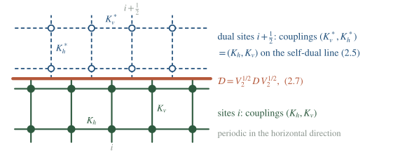
Figure 1. A horizontal duality line splices the lattice (below) to its dual (above), displaced by half a spacing. On the self-dual line (2.5) both sides carry the same couplings, and the dressed line commutes with the row transfer matrix, (2.8).

Two horizontal lines fuse into one row. The adjoint of the first relation in (2.6) is $V_1{D}^{†}=c{D}^{†}{V}_2$, so $D^{†}{V}_{2}D=c^{-1}{V}_1{D}^{†}D=c^{-1}{V}_1(1+\eta )$, and since η commutes with $V_1$ and $V_2$,

$${\mathcal{D}}^{†}\mathcal{D}=c^{-1}(1+\eta )\mathbb{T},\text{\hspace{1em}(2.9)}$$

which we checked for $L=3,4,5$; F2 explains the full row of the lattice that accompanies $1+\eta$.

2.3 Order and disorder [Proved.]

Multiplying the defining relations along a segment $a<b$ of the ring gives

$$D{\sigma }_a^z{\sigma }_b^z=\left(\prod _{j=a+1}^b{\sigma }_j^x\right)D,D\prod _{j=a+1}^b{\sigma }_j^x={\sigma }_{a+1}^z{\sigma }_{b+1}^{z}D.\text{\hspace{1em}(2.10)}$$

The product of ${\sigma }^x$ is the η segment between the dual sites $a+\frac{1}{2}$ and $b+\frac{1}{2}$, the Kadanoff–Ceva disorder pair of Sem I Week 4 §4.1 in Hamiltonian form, (3.10) of Sem II Week 4. The line therefore exchanges the order and disorder algebras, and two passages return the order pair translated by one site, as $D^2=(1+\eta )T$ requires. A single spin behaves differently. Since $D\eta =D$ and $\eta {\sigma }_a^z=-{\sigma }_a^z\eta$, we have $D{\sigma }_a^z(1+\eta )=0$: the operator $D{\sigma }_a^z$ vanishes on even states and maps the odd sector into the even one, with rank $2^{L-1}$ (checked at $L=4$). No local operator $X$ satisfies $D{\sigma }_a^z=XD$, since $XD$ vanishes on odd states. In spacetime, an order operator carried through the line emerges as a disorder operator attached to an η line that ends on $D$ [Heuristic reading of the identity; CCHLS §2.3 state the $3+1$d analogue].

3. The vertical line from half-space gauging

To lay the line along time we need the Hilbert space with the line inserted at one point of space. We derive it from gauging, following Sem II Week 4 §3.6 with the gauging restricted to part of space.

3.1 Gauging on an interval with Dirichlet ends [Proved.]

Take the ring of $L$ sites with $H(g)$ of conventions §4 and an interval $I=\{a+1,\dots ,b\}$ with $b-a\ge 2$. Put gauge qubits on the links inside $I$, at $a+\frac{3}{2},\dots ,b-\frac{1}{2}$, couple them as in Sem II Week 4 (3.2), and impose Gauss’s law at the interior sites only:

$$H_I(g)=-g\sum _{j=1}^L{\sigma }_j^x-\sum _{j\notin \{a+1,\dots ,b-1\}}{\sigma }_j^z{\sigma }_{j+1}^z-\sum _{j=a+1}^{b-1}{\sigma }_j^z{Z}_{j+\frac{1}{2}}{\sigma }_{j+1}^z,G_j=X_{j-\frac{1}{2}}{\sigma }_j^x{X}_{j+\frac{1}{2}}=1(a+2\le j\le b-1).\text{\hspace{1em}(3.1)}$$

The end sites carry no Gauss law and the end links $a+\frac{1}{2}$, $b+\frac{1}{2}$ carry no gauge qubit: the gauge field and the gauge parameter vanish at the ends, a Dirichlet condition. The condition is forced (F4), since with no qubit on the link $a+\frac{1}{2}$ a Gauss operator at $a+1$ would be ${\sigma }_{a+1}^x{X}_{a+3/2}$, which anticommutes with the bond ${\sigma }_a^z{\sigma }_{a+1}^z$. The physical space has dimension $2^{L+(b-a-1)-(b-a-2)}=2^{L+1}$. The Wilson line across the interval,

$$W_I=\prod _{j=a+1}^{b-1}{Z}_{j+\frac{1}{2}},\text{\hspace{1em}(3.2)}$$

commutes with $H_I$ and with every $G_j$, each of which contains two of its anticommuting partners. Fix the gauge by using $G_{a+2},\dots ,G_{b-1}$ in turn to set $Z_{a+3/2}=\cdots =Z_{b-3/2}=1$: each gauge orbit contains exactly one such configuration, the transverse fields do not act on links and preserve the condition, and the last link carries $Z_{b-1/2}=W_I$. The bond $(b-1,b)$ is then multiplied by $W_I$, every other term is that of $H(g)$, and

$$H_I(g){|}_{\mathrm{phys}}\cong H_0(g)\oplus H_1(g),\text{\hspace{1em}(3.3)}$$

where $H_0$ is the periodic chain and $H_1$ the antiperiodic one of Sem II Week 4 §3.1, each with all its states. Nothing projects onto η-even states, because constant gauge transformations are excluded by the Dirichlet ends; the sum over $W_I=\pm 1$ is the sum over the relative cohomology of the strip, $H^1(I\times \mathbb{R},\partial I\times \mathbb{R};{\mathbb{Z}}_2)={\mathbb{Z}}_2$, with unit weight. We built (3.1) with its Gauss projector for six choices of $(L,a,b)$ with $L=3,\dots ,6$, at $g=0.6$, 1 and 1.7, and the spectrum equals that of $H_0\oplus H_1$ to $10^{-13}$.

3.2 The two interfaces [Proved; checked numerically.]

On the interval we use the dual variables of Sem II Week 4 (3.5), ${\mu }_{j+1/2}^z=X_{j+1/2}$ and ${\mu }_{j+1/2}^x={\sigma }_j^z{Z}_{j+1/2}{\sigma }_{j+1}^z$ for $a+1\le j\le b-1$, together with two end qubits,

$${\tilde{\sigma }}_{a+1}^x={\sigma }_{a+1}^x{X}_{a+\frac{3}{2}},{\tilde{\sigma }}_{a+1}^z={\sigma }_{a+1}^z;{\tilde{\sigma }}_b^x=X_{b-\frac{1}{2}}{\sigma }_b^x,{\tilde{\sigma }}_b^z={\sigma }_b^z.$$

Each pair is a Pauli algebra, and it commutes with the μ’s (the factor $X$ compensates the anticommutation of ${\sigma }^x$ with the ${\sigma }^z$ inside ${\mu }^x$) and with every $G_j$. With the spins outside $I$ these are $L+1$ qubits, matching $2^{L+1}$. On physical states ${\sigma }_j^x={\mu }_{j-1/2}^z{\mu }_{j+1/2}^z$ for $a+2\le j\le b-1$ by Gauss’s law, while ${\sigma }_{a+1}^x={\tilde{\sigma }}_{a+1}^x{\mu }_{a+3/2}^z$ and ${\sigma }_b^x={\mu }_{b-1/2}^z{\tilde{\sigma }}_b^x$ by definition. Therefore

$$H_I=H_{\mathrm{out}}-{\sigma }_a^z{\tilde{\sigma }}_{a+1}^z-g{\tilde{\sigma }}_{a+1}^x{\mu }_{a+\frac{3}{2}}^z-\sum _{j=a+1}^{b-1}{\mu }_{j+\frac{1}{2}}^x-g\sum _{j=a+2}^{b-1}{\mu }_{j-\frac{1}{2}}^z{\mu }_{j+\frac{1}{2}}^z-g{\mu }_{b-\frac{1}{2}}^z{\tilde{\sigma }}_b^x-{\tilde{\sigma }}_b^z{\sigma }_{b+1}^z,\text{\hspace{1em}(3.4)}$$

where $H_{\mathrm{out}}$ contains the transverse fields $g{\sigma }_j^x$ outside $I$ and the bonds between consecutive sites outside $I$. Read around the ring, the terms of (3.4) form a cycle of anticommuting neighbours whose coefficients alternate $g,1,g,1,\dots$ without interruption at the ends (Figure 2); inside $I$ the coefficient $g$ multiplies the bonds of the μ chain, which is therefore $gH(1/g)$. The ends are interfaces between $H(g)$ and $gH(1/g)$, with the patterns

$$(\dots ,{\sigma }_a^x,{\sigma }_a^z{\tilde{\sigma }}_{a+1}^z,{\tilde{\sigma }}_{a+1}^x{\mu }_{a+\frac{3}{2}}^z,{\mu }_{a+\frac{3}{2}}^x,\dots )\text{and}(\dots ,{\mu }_{b-\frac{1}{2}}^x,{\mu }_{b-\frac{1}{2}}^z{\tilde{\sigma }}_b^x,{\tilde{\sigma }}_b^z{\sigma }_{b+1}^z,{\sigma }_{b+1}^x,\dots ),\text{\hspace{1em}(3.5)}$$

in which the end qubit has a bond on one side, a mixed term on the other, and no transverse field; the second pattern is the mirror image of the first. We diagonalized (3.4) for the cases of §3.1 and found the spectrum of $H_0\oplus H_1$ to $10^{-13}$.

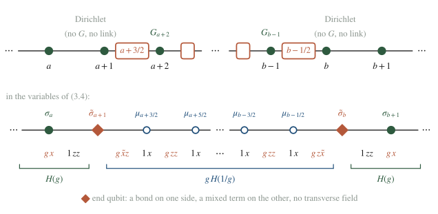
Figure 2. Gauging on an interval with Dirichlet ends (top) and the same chain in the variables of (3.4) (bottom). The coefficients alternate g, 1 across both interfaces; inside the interval g multiplies bonds, so the μ chain is gH(1/g), and each end qubit ◆ lacks a transverse field.

3.3 One line on the ring, and its motion [Computed.]

At $g=1$ both regions of (3.4) are the critical chain, and each interface is visible only through the term it lacks. A single interface of the first pattern can therefore be closed on the ring. With the line at site $d$,

$$H_D^{(d)}=-\sum _{j\ne d}{\sigma }_j^x-\sum _{j\ne d}{\sigma }_j^z{\sigma }_{j+1}^z-{\sigma }_d^x{\sigma }_{d+1}^z,\text{\hspace{1em}(3.6)}$$

a cycle of $2L-1$ terms instead of the $2L$ of the periodic chain (Figure 3). For $L=3$ and $d=3$, in the basis $|s_1{s}_2{s}_3⟩$ with index $4s_1+2s_2+s_3$,

$$H_D^{(3)}=\left(\begin{array}{cccccccc}-2& -1& -1& 0& -1& 0& 0& 0\\ -1& 0& 0& -1& 0& -1& 0& 0\\ -1& 0& 2& -1& 0& 0& -1& 0\\ 0& -1& -1& 0& 0& 0& 0& -1\\ -1& 0& 0& 0& 0& 1& -1& 0\\ 0& -1& 0& 0& 1& 2& 0& -1\\ 0& 0& -1& 0& -1& 0& 0& 1\\ 0& 0& 0& -1& 0& -1& 1& -2\end{array}\right),$$

with eigenvalues $\pm 3.077684$ and $\pm 0.726543$, each twice. AMF’s duality-twisted chain (3.37) at $J=1$ is the mirror image of (3.6) with the defect spin rotated, ${\sigma }^x\to {\sigma }^y$ [Stated — refs: AMF §3.4].

The line moves by a two-site unitary. Let $U_d={\mathsf{H}}_{d+1}{\mathrm{CZ}}_{d,d+1}$, with $\mathsf{H}$ the Hadamard gate and $\mathrm{CZ}=\mathrm{diag}(1,1,1,-1)$ in the basis $|s_d{s}_{d+1}⟩$. Then

$$U_d=\frac{1}{\sqrt{2}}\left(\begin{array}{cccc}1& 1& 0& 0\\ 1& -1& 0& 0\\ 0& 0& 1& -1\\ 0& 0& 1& 1\end{array}\right),{\sigma }_d^z\mapsto {\sigma }_d^z,{\sigma }_d^x\mapsto {\sigma }_d^x{\sigma }_{d+1}^x,{\sigma }_{d+1}^z\mapsto {\sigma }_{d+1}^x,{\sigma }_{d+1}^x\mapsto {\sigma }_d^z{\sigma }_{d+1}^z,\text{\hspace{1em}(3.7)}$$

where the map is $O\mapsto U_{d}O{U}_d^{†}$: CZ sends ${\sigma }_d^x\to {\sigma }_d^x{\sigma }_{d+1}^z$ and ${\sigma }_{d+1}^x\to {\sigma }_d^z{\sigma }_{d+1}^x$, fixing both ${\sigma }^z$, and the Hadamard then exchanges ${\sigma }_{d+1}^x$ and ${\sigma }_{d+1}^z$. The terms of (3.6) that involve sites $d$ and $d+1$ go to

$${\sigma }_{d-1}^z{\sigma }_d^z\mapsto {\sigma }_{d-1}^z{\sigma }_d^z,{\sigma }_d^x{\sigma }_{d+1}^z\mapsto {\sigma }_d^x,{\sigma }_{d+1}^x\mapsto {\sigma }_d^z{\sigma }_{d+1}^z,{\sigma }_{d+1}^z{\sigma }_{d+2}^z\mapsto {\sigma }_{d+1}^x{\sigma }_{d+2}^z,$$

and the others are untouched, which is the term list of $H_D^{(d+1)}$:

$$U_d{H}_D^{(d)}{U}_d^{†}=H_D^{(d+1)}.\text{\hspace{1em}(3.8)}$$

We checked (3.8) for every $d$, including $d=L$, for $L=3,\dots ,6$. The position of the line is unobservable, and with (2.8) the line is topological in both directions of spacetime at the self-dual point.

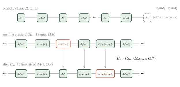
Figure 3. The terms of the critical chain as a cycle of anticommuting neighbours. The duality line replaces the transverse field and the bond of one site by a single mixed term, and the two-site unitary (3.7) moves the replacement by one site.

3.4 Fusion and absorption in both channels [Proved; checked numerically.]

In the horizontal channel the fusion is the operator identity $D^{†}D=1+\eta$ of Sem II Week 4 §3.6, or (2.9) on the transfer matrix, and the absorption is $D\eta =\eta D=D$. In the vertical channel the fusion is a statement about Hilbert spaces. At $g=1$ the interval-gauged ring of §3.2 is a ring of $L+1$ qubits carrying two duality lines, of the two patterns (3.5), and (3.3) states that

$$\mathrm{spec}{H}_{D,\bar{D}}(L+1\text{qubits})=\mathrm{spec}{H}_0(L)\bigsqcup \mathrm{spec}{H}_1(L),\text{that is,}{\mathcal{H}}_{D\times \bar{D}}={\mathcal{H}}_1\oplus {\mathcal{H}}_{\eta },\text{\hspace{1em}(3.9)}$$

the untwisted and the η-twisted Hilbert spaces of the chain of $L$ sites: $D\times \bar{D}=1+\eta$. Two lines of the same pattern (3.6), on rings of $L+1=4,5,6$ qubits at neighbouring and at separated sites, give the same union to $10^{-14}$; in every case the pair of lines removes one site (F2).

For the absorption, put an η twist, a flipped bond (the Kadanoff–Ceva seam of Sem I Week 4 §4.1), on the bond $(d-1,d)$ next to the line, $H_{D,\eta }=H_D^{(d)}+2{\sigma }_{d-1}^z{\sigma }_d^z$. The operator ${\sigma }_d^x$ flips the sign of ${\sigma }_{d-1}^z{\sigma }_d^z$ and commutes with every other term of (3.6), since the site $d$ has neither a transverse field nor a bond to its right, so

$${\sigma }_d^x{H}_{D,\eta }{\sigma }_d^x=H_D^{(d)}.\text{\hspace{1em}(3.10)}$$

A twist elsewhere is brought next to the line by the seam moves of Sem I Week 4 §4.1, so ${\mathcal{H}}_{D\times \eta }\cong {\mathcal{H}}_D$: $D\times \eta =D$. The seam ends on the line at no cost and its endpoint, the disorder operator, is absorbed; on a ring without a line the same conjugation only moves the twist.

3.5 What a numerical diagonalization shows [Computed; the conformal dimensions Stated — refs: Shao §3.1.1.]

Physical picture. Every level of $H_D^{(d)}$ is exactly doubly degenerate ($L=3,\dots ,8$), which Problem 4 traces to an antiunitary symmetry, as AMF (3.38)–(3.39) do. The ground-state energy exceeds that of the periodic chain by $E_D-E_P=2/\pi +\pi /(4L)+O(L^{-2})$: at $L=16$, $L(E_D-E_P)-2L/\pi =0.7945$ against $\pi /4=0.7854$, and for the antiperiodic chain $L(E_A-E_P)=1.5721$ against $\pi /2=1.5708$. The constant $2/\pi$ is local, the energy $-2/\pi$ per term of the bulk energy $-4L/\pi$ that the line removes. The $1/L$ terms are universal: with the velocity $v=2$ of $H(1)$, $\pi /(4L)=(2\pi v/L)\cdot \frac{1}{16}$ and $\pi /(2L)=(2\pi v/L)\cdot \frac{1}{8}$, the dimensions of the lowest duality-twisted state, $(h,\bar{h})=(\frac{1}{16},0)$, and of the disorder field, $(\frac{1}{16},\frac{1}{16})$, of the Ising CFT. The quantum dimension is visible too: $D|0⟩=\sqrt{2}|0⟩$ on the ground state of $H(1)$ for $L=3,\dots ,8$, while at $g=0.8$, $L=6$, $|0⟩$ is no eigenvector and $⟨0|D|0⟩=1.2978$. The twisted ring is a closed chain of $2L-1$ Majorana operators with one unpaired mode (Problem 5⋆), which AMF find localized on the domain wall away from criticality (their §3.4).

Everything in §§2–3 used one property of the Ising chain: gauging its ${\mathbb{Z}}_2$ returns the same chain at the dual coupling. The next section isolates this property.

4. Half-space gauging as the general mechanism [The count (4.2)–(4.3) Proved, given (4.1); topological invariance Proved for the chain and Sketched in general.]

Let $\mathcal{T}$ be a theory in $d$ dimensions with a non-anomalous ${\mathbb{Z}}_N^{(q)}$ symmetry, and suppose that at some coupling $\mathcal{T}\cong \mathcal{T}/{\mathbb{Z}}_N^{(q)}$ through a local map φ. Gauge ${\mathbb{Z}}_N^{(q)}$ in a region $R$ with boundary $M$, summing over $B\in Z^{q+1}(R;{\mathbb{Z}}_N)$ with the normalization (2.5) of Sem II Week 4, with $B$ and the gauge parameters vanishing on $M$ (Dirichlet). The result is $\mathcal{T}$ outside $R$ and $\mathcal{T}/{\mathbb{Z}}_N^{(q)}$ inside, glued along $M$, and composing with φ inside gives a defect $D(M)$ of $\mathcal{T}$. Section 3 is the case $d=2$, $q=0$, $N=2$, with $R$ an interval times time and φ the relabeling $R$ of Sem II Week 4 §3.6.

Topological invariance. The summed field is flat, so gauging changes no local dynamics; enlarging $R$ by one cell adds one gauge variable and one Gauss constraint, an isometry that, composed with φ, moves $D$. In the chain this is (3.7)–(3.8); in general φ must be local, as the exact dualities of Sem II Week 12 are.

Fusion. $D(M)\times \bar{D}(M)$ is the gauging in the slab $M\times I$ with Dirichlet conditions on both faces. The relative cohomology of the slab is that of $M$ shifted by one degree,

$$H^k(M\times I,M\times \partial I;{\mathbb{Z}}_N)\cong H^{k-1}(M;{\mathbb{Z}}_N),\text{\hspace{1em}(4.1)}$$

by the Künneth formula for the pair $(I,\partial I)$, whose only nonzero group is $H^1(I,\partial I;\mathbb{Z})=\mathbb{Z}$; CCHLS reach the same groups through Lefschetz duality. In the normalization of Sem II Week 4 (2.5) the sum runs over $[B]\in H_{\mathrm{rel}}^{q+1}\cong H^q(M)$, and the prefactor uses relative groups, because the gauge parameters vanish on the faces: $|H_{\mathrm{rel}}^{q-1}||H_{\mathrm{rel}}^{q-3}|\cdots /(|H_{\mathrm{rel}}^q||H_{\mathrm{rel}}^{q-2}|\cdots )=|H^{q-2}(M)||H^{q-4}(M)|\cdots /(|H^{q-1}(M)||H^{q-3}(M)|\cdots )$. Each class of $H^q(M)$ is Poincaré dual, in the closed oriented $(d-1)$-manifold $M$, to a cycle $\Sigma \in H_{d-1-q}(M;{\mathbb{Z}}_N)$ on which it inserts the symmetry operator $\eta (\Sigma )$. Therefore

$$D\times \bar{D}=C_q(M)\equiv \frac{|H^{q-2}(M)||H^{q-4}(M)|\cdots }{|H^{q-1}(M)||H^{q-3}(M)|\cdots }\sum _{\Sigma \in H_{d-1-q}(M;{\mathbb{Z}}_N)}\eta (\Sigma ),\text{\hspace{1em}(4.2)}$$

and for connected $M$

$$q=0:D\times \bar{D}=\sum _{k=0}^{N-1}{\eta }^k;q=1:D\times \bar{D}=\frac{1}{N}\sum _{\Sigma \in H_{d-2}(M;{\mathbb{Z}}_N)}\eta (\Sigma ).\text{\hspace{1em}(4.3)}$$

For $d=2$ and $N=2$ the first is $1+\eta$, (3.9), with the unit coefficients of the Dirichlet strip of §3.1. For $d=4$ the second is CCHLS (2.17)–(2.19), including their normalization $x=1/N$, (2.18). For $d=3$ it is the gauging of ${\mathbb{Z}}_N^{(1)}$ on the surface $M$ itself: the slab has collapsed to a condensation defect.

Absorption. In $\mathcal{T}/{\mathbb{Z}}_N^{(q)}$ an insertion of $\eta (\Sigma )$ shifts the summed background by the class dual to Σ, a relabeling of the sum, so the operators of the gauged symmetry act trivially there. An η brought into $R$ from outside therefore disappears, $\eta \times D=D\times \eta =D$, which is (3.10) in the chain.

The right side of (4.2) needs no self-duality: it is the gauging of ${\mathbb{Z}}_N^{(q)}$ on a manifold of codimension one, a topological defect of any theory with a suitable symmetry (§5).

5. A condensation defect in $2+1$d ${\mathbb{Z}}_N$ gauge theory

5.1 The sheet as higher gauging [Proved.]

Take ${\mathbb{Z}}_N$ gauge theory at its BF point (Sem II Week 2; the toric code of Sem II Week 8 for $N=2$), whose higher-form-symmetries in $d=3$ are both 1-form (conventions §6): the Wilson lines $W_e={\omega }^{e\oint a}$, carrying the charges $e^e$, generate the magnetic ${\mathbb{Z}}_N^{(1)}$ and act on the ‘t Hooft lines ($b$-lines, carrying the fluxes $m^s$) by ${\omega }^{es\mathrm{Link}}$, and the ‘t Hooft lines generate the electric one (conventions §7). A sheet of condensed electric charge is a surface Σ on which the worldlines of the charges in a subgroup

$$H=⟨k⟩=r{\mathbb{Z}}_N\cong {\mathbb{Z}}_{N^{\prime }},r=\gcd (N,k),N^{\prime }=N/r,\mathrm{Ann}(H)=N^{\prime }{\mathbb{Z}}_N\cong {\mathbb{Z}}_r,$$

proliferate freely, in the notation of Sem II Week 4 §5.1. In the language of RSS this is the higher gauging of the subgroup $H$ of the magnetic ${\mathbb{Z}}_N^{(1)}$ on Σ: one sums over networks of the lines of $H$ drawn on Σ, which behave as the lines of a 0-form symmetry of the two-dimensional surface (RSS §3.2). The normalization is (4.2) with $q=1$ and ${\mathbb{Z}}_N$ replaced by $H$:

$$S_H(\Sigma )=\frac{1}{|H^0(\Sigma ;H)|}\sum _{\gamma \in H_1(\Sigma ;H)}W(\gamma ),\text{\hspace{1em}(5.1)}$$

where $W(\gamma )$ is the Wilson line with $H$-valued charge along the cycle γ. RSS normalize by $1/\sqrt{|H_1(\Sigma ;H)|}$ instead, their (5.4) and (5.11); the two agree on the torus and differ by $|H{|}^{g-1}$ on a surface of genus $g$, an Euler counterterm (F7).

Orientation reversal sends γ to $-\gamma$, so ${\bar{S}}_H=S_H$; and the condensed lines are pure charges, with trivial spin and mutual braiding (conventions §9), so parallel copies fuse without phases, $W(\gamma )W({\gamma }^{\prime })=W(\gamma +{\gamma }^{\prime })$, which is RSS (5.8) at trivial spin. Therefore

$$S_H\times {\bar{S}}_H=\frac{1}{|H^0{|}^2}\sum _{\gamma ,{\gamma }^{\prime }}W(\gamma +{\gamma }^{\prime })=\frac{|H_1(\Sigma ;H)|}{|H^0(\Sigma ;H){|}^2}\sum _{\gamma }W(\gamma )=Z_H(\Sigma )S_H(\Sigma ),Z_H({\Sigma }_g)=\frac{|H_1({\Sigma }_g;H)|}{|H^0({\Sigma }_g;H)|}=|H{|}^{2g-1},\text{\hspace{1em}(5.2)}$$

where $Z_H(\Sigma )$ is the partition function of the two-dimensional $H$ gauge theory on Σ in the normalization of Sem II Week 4 (2.5), the $1+1$d coefficient of RSS (5.12). The normalized sheet $P_H=S_H/Z_H(\Sigma )$ is idempotent, and $S_H$ has no inverse unless $H$ is trivial.

5.2 The lattice sheet on a time slice [Computed.]

On a time slice the sheet is an operator. Cellulate Σ by a square lattice Λ with $N_s$ sites, $N_{\ell }$ links and $N_P$ plaquettes, put the clock and shift of conventions §4 on the links, with the Gauss operators $G_x$ and plaquette operators $B_P$ of Sem II Week 2 §6.4, and let $W(c)={\prod }_{\ell }{Z}_{\ell }^{c_{\ell }}$ for $c\in C_1(\Lambda ;H)$. We define

$$S_H=|H{|}^{-N_P}\sum _{c\in Z_1(\Lambda ;H)}W(c).\text{\hspace{1em}(5.3)}$$

On the flux-free subspace a boundary acts trivially, $W(\partial f)={\prod }_P{B}_P^{\pm f_P}=1$, so all $|B_1(\Lambda ;H)|=|H{|}^{N_P}/|Z_2(\Lambda ;H)|=|H{|}^{N_P-1}$ cycles of a homology class act alike, and (5.3) reduces to (5.1).

To evaluate (5.3) in the basis $|a⟩$ of link variables, where $W(c)|a⟩={\omega }^{⟨c,a⟩}|a⟩$, write $c=r\bar{c}$ with $\bar{c}\in Z_1(\Lambda ;{\mathbb{Z}}_{N^{\prime }})$. The sum ${\sum }_{\bar{c}}{e}^{2\pi i⟨\bar{c},a⟩/N^{\prime }}$ equals $|Z_1(\Lambda ;{\mathbb{Z}}_{N^{\prime }})|$ if $⟨\bar{c},a⟩\equiv 0$ mod $N^{\prime }$ for every cycle $\bar{c}$, and 0 otherwise. The cochains that annihilate all cycles are the coboundaries, by the perfectness of the pairing used in Sem II Week 4 §4.2, so the condition is $a$ mod $N^{\prime }\in B^1(\Lambda ;{\mathbb{Z}}_{N^{\prime }})$: every plaquette flux $(da{)}_P$ and every holonomy of $a$ lies in $N^{\prime }{\mathbb{Z}}_N=\mathrm{Ann}(H)$. With $|Z_1(\Lambda ;{\mathbb{Z}}_{N^{\prime }})|=|H{|}^{N_{\ell }-N_s+1}=|H{|}^{N_P+2g-1}$,

$$S_H=Z_H(\Sigma ){\Pi }_H,\text{\hspace{1em}(5.4)}$$

where ${\Pi }_H$ is the projector onto the link configurations whose fluxes and holonomies all lie in $\mathrm{Ann}(H)$. Thus $S_H^2=Z_H{S}_H$ and $S_H^{†}=S_H$ as operators. $S_H$ commutes with every $B_P$, both being diagonal, and with every $G_x$, which shifts the link variables by a coboundary and changes no flux and no holonomy; therefore it commutes with the BF Hamiltonian $H_{\mathrm{TC}}=-{\sum }_x\mathrm{Re}{G}_x-{\sum }_P\mathrm{Re}{B}_P$ of Sem II Week 2 §6.4, the time-slice form of its topological invariance.

The action on lines follows from (5.4).

(i) ‘t Hooft lines through the sheet. A flux $m^s$ at a plaquette $P$ is an ‘t Hooft line piercing the time slice. ${\Pi }_H$ annihilates the state unless $s\in \mathrm{Ann}(H)$: the cycles $c$ and $c+h\partial P$ enter (5.3) together, and ${\sum }_{h\in H}{\omega }^{hs}=|H|{\delta }_{s\in \mathrm{Ann}(H)}$, the small condensed loop around the puncture of Figure 4. The flux passes if a line of the dual symmetry is attached to it on the sheet. Let γ̃ be a dual path from $P^{\prime }$ to $P$ and ${\lambda }_{\tilde{\gamma }}$ the signed indicator of the links it crosses, so that $d{\lambda }_{\tilde{\gamma }}$ is $+1$ at $P$ and $-1$ at $P^{\prime }$, and define

$$S_H^{[s,\tilde{\gamma }]}=|H{|}^{-N_P}\sum _{c\in Z_1(\Lambda ;H)}{\omega }^{-s⟨c,{\lambda }_{\tilde{\gamma }}⟩}W(c)=Z_H(\Sigma ){\Pi }_H^{[s,\tilde{\gamma }]},\text{\hspace{1em}(5.5)}$$

where ${\Pi }_H^{[s,\tilde{\gamma }]}$ projects onto the $a$ for which $a-s{\lambda }_{\tilde{\gamma }}$ has all fluxes and holonomies in $\mathrm{Ann}(H)$; these include the flux pair $(s,-s)$ at $(P,P^{\prime })$. Since $c\in r\mathbb{Z}$, the phase depends on $s$ only through ${\mathrm{res}}_H(s)\in \hat{H}$: (5.5) is the sheet carrying a line of the dual symmetry $\hat{H}\cong {\mathbb{Z}}_{N^{\prime }}$ along γ̃, the higher quantum symmetry of RSS §3.4.

(ii) Wilson lines. $S_H$ commutes with every $W(\gamma )$ and $G_x$, so charges pass. $W(c)S_H=S_H$ for $c\in Z_1(\Lambda ;H)$, and for an open $H$-valued chain γ, $S_{H}W(\gamma )$ depends only on $\partial \gamma$: the condensed charges end on the sheet. For $e\notin H$, moving the chain across a flux $s\in \mathrm{Ann}(H)$ multiplies $S_H{W}_e(\gamma )$ by ${\omega }^{es}$, and $\mathrm{Ann}(\mathrm{Ann}(H))=H$, so these charges cannot end; across the sheet a Wilson charge is conserved modulo $H$.

(iii) The action of RSS §3.3. RSS define $S\cdot L$ by wrapping the sheet around a tube that encloses $L$, an action captured by the Hilbert space of the torus. On the ground space of $H_{\mathrm{TC}}$ let $|1⟩$ have $W(C_x)=U({\tilde{C}}_x)=1$, and $|e^a{m}^b⟩=U({\tilde{C}}_y{)}^{b}W(C_y{)}^a|1⟩$ with the holonomies of Sem II Week 2 (6.13): the line $e^a{m}^b$ along the core of the solid torus with meridian $C_x$. Since $W(C_x)U({\tilde{C}}_y)=\omega U({\tilde{C}}_y)W(C_x)$ (Sem II Week 2, Figure 5), $W(C_x{)}^h|e^a{m}^b⟩={\omega }^{hb}|e^a{m}^b⟩$, the braiding of the meridian loop with the core, while $W(C_y{)}^h|e^a{m}^b⟩=|e^{a+h}{m}^b⟩$. On the torus (5.1) is $|H{|}^{-1}{\sum }_{h_1,h_2\in H}W(C_x{)}^{h_1}W(C_y{)}^{h_2}$, so

$$S_H\cdot e^a{m}^b={\delta }_{b\in \mathrm{Ann}(H)}\sum _{h\in H}{e}^{a+h}{m}^b.\text{\hspace{1em}(5.6)}$$

5.3 $N=4$, $H=⟨2⟩$ on the $2\times 2$ torus [Computed.]

Here $r=N^{\prime }=2$ and $H=\mathrm{Ann}(H)=\{0,2\}$. The $2\times 2$ torus has 8 links, 4 plaquettes and $4^8=65536$ states, and $Z_1(\Lambda ;H)=2Z_1(\Lambda ;{\mathbb{Z}}_2)$ has $2^{N_P+1}=32$ elements, so (5.3) is $2^{-4}$ times their sum. Built as a matrix on the 65536 states, $S_H$ has eigenvalues 0 and 2, and $S_H^2=2S_H$, $[S_H,G_x]=0$ and $S_H=2{\Pi }_H$ hold exactly. The ground space of $H_{\mathrm{TC}}$ has 16 states, each uniform over a gauge orbit of 64 flat configurations, and $S_H=2$ on the four with both holonomies even. In the basis $|e^a{m}^b⟩$ of §5.2(iii), with $b$ the slow index,

$$S_H{|}_{\mathrm{GS}}=\mathrm{diag}(1,0,1,0{)}_b\otimes {\left(\begin{array}{cccc}1& 0& 1& 0\\ 0& 1& 0& 1\\ 1& 0& 1& 0\\ 0& 1& 0& 1\end{array}\right)}_a,\text{\hspace{1em}(5.7)}$$

which is (5.6): $e^a{m}^b\mapsto e^a{m}^b+e^{a+2}{m}^b$ for $b\in \{0,2\}$, and 0 for $m$ and $m^3$; its trace is 8. A single link shifted by one unit carries the fluxes $(1,3)$ on its two plaquettes and is annihilated; shifted by two it carries $(2,2)$ and has $S_H=2$; the dressed sheet (5.5) with $s=1$, along the one-step dual path between the two plaquettes, has eigenvalue 2 on the $(1,3)$ configuration.

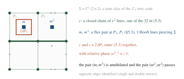
Figure 4. The condensation sheet on a time slice. The sum over all closed chains of condensed lines contains, with every chain, the same chain plus the small loop around a puncture; the two cancel for a flux outside Ann(H), (5.4).

5.4 The sheet in one box [Proved in §§5.1–5.3.]

For a subgroup $H=⟨k⟩$ of the charges of ${\mathbb{Z}}_N$ gauge theory, the condensation sheet on a closed oriented surface Σ is

$$\boxed{S_H(\Sigma )=\frac{1}{|H^0(\Sigma ;H)|}\sum _{\gamma \in H_1(\Sigma ;H)}W(\gamma ),S_H\times {\bar{S}}_H=Z_H(\Sigma )S_H,Z_H({\Sigma }_g)=|H{|}^{2g-1},}\text{\hspace{1em}(5.8)}$$

and $P_H=S_H/Z_H(\Sigma )$ is the projector onto the states on which every condensed line $W(\gamma )$, $\gamma \in H_1(\Sigma ;H)$, acts as 1. All Wilson lines pass; those with charge in $H$ end on the sheet, and across it a charge is conserved modulo $H$, so the labels that survive form ${\mathbb{Z}}_N/H\cong {\mathbb{Z}}_r$. ‘t Hooft lines with flux $s\in \mathrm{Ann}(H)\cong {\mathbb{Z}}_r$ pass; the others are annihilated, (5.4) and (5.6), unless the dual line of label ${\mathrm{res}}_H(s)\in \hat{H}\cong {\mathbb{Z}}_{N^{\prime }}$ is attached to them on the sheet, (5.5). The bookkeeping uses the sequence (5.1) of Sem II Week 4 for the fluxes and the quotient sequence for the charges,

$$0\to \mathrm{Ann}(H)\to {\mathbb{Z}}_N\to \hat{H}\to 0(\text{’t Hooft fluxes}),0\to H\to {\mathbb{Z}}_N\to {\mathbb{Z}}_N/H\to 0(\text{Wilson charges}).$$

Physical picture. The sheet is a charge-$k$ superconductor of zero thickness. A Wilson line of charge $h\in H$ ends on it because the condensate supplies the opposite charge. A flux $s$ threading it is seen by the condensate as the Aharonov–Bohm phase ${\omega }^{ks}$, which must be 1, so only $s\in \mathrm{Ann}(H)$ passes: flux quantization, with the Meissner effect of the sheet for the other fluxes. The identities are exact (§5.2), and the superconductor language is a heuristic reading. In Sem I Week 14 the same matter filled space and left the residual ${\mathbb{Z}}_r^{(1)}$, and Sem II Week 8 §7.3 identified $e$ condensation with Higgsing.

6. Duality defects in $3+1$ dimensions [Stated — refs: CCHLS §§2.3, 4.2, 5.2; KOZ; Koide–Nagoya–Yamaguchi. The fusion normalization is (4.3), proved in §4.]

For $d=4$ and $q=1$, a theory with a non-anomalous ${\mathbb{Z}}_N^{(1)}$ and $\mathcal{T}\cong \mathcal{T}/{\mathbb{Z}}_N^{(1)}$ has a three-dimensional duality defect with

$$\eta \times D=D\times \eta =D,D\times \bar{D}=\frac{1}{N}\sum _{S\in H_2(M;{\mathbb{Z}}_N)}\eta (S),\text{\hspace{1em}(6.1)}$$

CCHLS (2.19). The $\eta (S)$ are the surface operators of the 1-form symmetry (conventions §6), and the right side is their condensation on the worldvolume $M$, the $3+1$d counterpart of $1+\eta$. CCHLS also find $⟨D⟩=1/\sqrt{N}$ on $S^3$, their (2.20), and that sweeping $D$ past a line charged under ${\mathbb{Z}}_N^{(1)}$ attaches a ${\mathbb{Z}}_N$ surface to it. For Maxwell theory the composite of the exact self-duality (3.4) and the exact gauging (4.4) of Sem II Week 12 fixes $\beta =N/2\pi$, $e^2=2\pi /N$, the point $\tau =iN$ in the normalization of CCHLS (4.6), where CCHLS construct the defect in the continuum (§4.2) and on the modified Villain lattice as a Chern–Simons coupling (§5.2). KOZ obtain the same fusion rules for gauge theories that are self-dual under gauging, among them $SO(3)$ Yang–Mills theory at $\theta =\pi$ and $\mathcal{N}=4$ $SU(2)$ super-Yang–Mills theory at $\tau =i$, and Koide, Nagoya and Yamaguchi built the defect of Wegner’s four-dimensional ${\mathbb{Z}}_2$ lattice gauge theory at its self-dual point (conventions §4) in the manner of AMF. Problem 8⋆⋆ asks for the Hamiltonian version.

7. Mini-calculation 5 (hand-in)

7.1 Scope

The calculation is exact on finite rings and on the row transfer matrix along the self-dual line (2.5); it uses §§2–3 and Sem II Week 4 §3. Nothing is claimed about the continuum, except in the optional Sub-task 5, which imports the Ising CFT dimensions of Shao §3.1.1 to name what the finite-size numbers measure.

7.2 Variable dictionary

symbol	meaning	where
${\sigma }_i^{x,z}$, $\eta ={\prod }_i{\sigma }_i^x$	Ising spins on the ring; the ${\mathbb{Z}}_2$ line	conventions §4
$D$	Kramers–Wannier operator, $D^{†}D=1+\eta$, $D^2=(1+\eta )T$	Sem II Week 4 (3.12)
$V_1,V_2,\mathbb{T}$	vertical and horizontal bond factors, row transfer matrix	(2.1)
$\mathcal{D}$	horizontal line on the transfer matrix	(2.7)
${\prod }_{j=a+1}^b{\sigma }_j^x$	Kadanoff–Ceva disorder pair, an η segment	(2.10)
$H_I$, $H_D^{(d)}$, $U_d$, $H_{D,\eta }$	interval-gauged chain; ring with one line; the move; line plus seam	(3.1), (3.6)–(3.7), (3.10)

7.3 Sub-tasks

Sub-task 1: the line on the four-site transfer matrix. Build $D$ for $L=4$ from Sem II Week 4 (3.12) and display $4D$ as a $16\times 16$ sign matrix. Build $V_1(K_v)$ and $V_2(K_h)$ at $K_v=0.3$, $K_h=K_v^{\ast }$, the row $\mathbb{T}$ and the line $\mathcal{D}$; verify (2.3), (2.6), (2.8) and (2.9), and evaluate $[\mathcal{D},\mathbb{T}]$ at $(K_h,K_v)=(0.5,0.3)$. Deliverable: the matrix and the residuals. Checkpoint: $K_v^{\ast }=0.616679$ and $\sinh 2K_h\sinh 2K_v=1$; $D$ has rank 8; the residuals of (2.6), (2.8) and (2.9) are of order $10^{-15}$ relative to $\mathbb{T}$; at $(0.5,0.3)$ the largest entry of $[\mathcal{D},\mathbb{T}]$ is 0.197 of the largest entry of $\mathbb{T}$; on the ground state of $H(1)$, with $E_0=-5.226252=-2\csc (\pi /8)$, $D|0⟩=\sqrt{2}|0⟩$.

Sub-task 2: order and disorder. Verify (2.10) for the six pairs $a<b$ of the four-site ring, verify $D{\sigma }_1^z(1+\eta )=0$, and compute the rank of $D{\sigma }_1^z$. Deliverable: the residuals, the rank, and one paragraph on why no local $X$ satisfies $D{\sigma }_1^z=XD$. Checkpoint: the residuals vanish to machine precision and the rank is 8.

Sub-task 3: $D\times \bar{D}=1+\eta$ in both channels. In the horizontal channel verify $D^{†}D=1+\eta$ and (2.9) at $L=4$. In the vertical channel gauge the interval $\{2,3,4\}$ of the four-site ring ($a=1$, $b=4$) as in (3.1), with two link qubits and the Gauss law at site 3, and diagonalize on the 32-dimensional physical space; then diagonalize the five-qubit ring (3.4) at $g=1$, and the five-qubit ring with two lines of the pattern (3.6) at sites 1 and 3. Deliverable: the 32 levels of each construction and their comparison with $\mathrm{spec}{H}_0(4)\bigsqcup \mathrm{spec}{H}_1(4)$. Checkpoint: the six lowest levels are $-5.226252$, $-4.828427$ (twice), $-3.695518$ (twice) and $-2.164784$, with $-4.828427=-(2+2\sqrt{2})$, and the three constructions agree to $10^{-14}$.

Sub-task 4: the Kadanoff–Ceva line meets $D$. On the four-site ring with the line at $d=4$, flip each of the three bonds of (3.6) in turn and compare the spectra with that of $H_D^{(4)}$; verify (3.10) for the bond $(3,4)$; verify $D\eta =\eta D=D$ and $\mathcal{D}\eta =\eta \mathcal{D}=\mathcal{D}$. Deliverable: the spectra, the residuals, and one paragraph explaining why a single twist can be removed on the ring with a line and not on the ring without one. Checkpoint: the levels of $H_D^{(4)}$ are $\pm 4.381286$, $\pm 2.645751$, $\pm 1.253960$ and $\pm 0.481575$, each twice, with $4.381286=\cot (\pi /14)$ and $2.645751=\sqrt{7}$, for every position of the flipped bond.

Sub-task 5 (optional): finite-size spectroscopy. With a sparse eigensolver compute $E_P$, $E_A$ and $E_D$ for $L=8,10,\dots ,16$ and extract the twisted-sector dimensions with $v=2$. Deliverable: the table and the extrapolation. Checkpoint: $L(E_A-E_P)=1.57586$, 1.57304 and 1.57206, and $L(E_D-E_P)-2L/\pi =0.80542$, 0.79791 and 0.79448, at $L=8$, 12 and 16.

7.4 What is proved, modeled and imported

Proved on every finite ring: (2.2)–(2.10), (3.3), (3.8), (3.9) and (3.10), which are operator statements. Modeled: the vertical line lives in the Hamiltonian limit of the transfer matrix (§2.1), where (3.6) replaces AMF’s defect Boltzmann weights; the horizontal line is exact on the full transfer matrix. Computed: the numbers of Sub-tasks 1, 3, 4 and 5 and the rank in Sub-task 2. Imported: the conformal dimensions $\frac{1}{16}$ and $\frac{1}{8}$ of the twisted sectors of the Ising CFT, used only in Sub-task 5 to name what the finite-size gaps measure.

8. Seminar: Aasen–Mong–Fendley §§2–3

Format as in Sem II Week 4 §8; every student reads the sections beforehand and brings Problem 4.

Sections. AMF §2 (pp. 4–6) and §3 (pp. 6–17).

The technical claim. A defect line built from modified Boltzmann weights commutes with the transfer matrix when the weights obey local defect commutation relations, (3.17) for the duality defect. This defect splices the lattice to its dual and obeys $D_{\sigma }^2=1+D_{\psi }$ and $D_{\sigma }{D}_{\psi }=D_{\psi }{D}_{\sigma }=D_{\sigma }$, their (3.27), with $D_{\psi }$ the spin flip, so that its eigenvalues are 0 and $\pm \sqrt{2}$.

What it needs from Semester I. Sem I Week 4 §§3–4, and §2.1 here.

The step at the board. The fusion (3.25)–(3.26) in AMF’s variables, with the hatted spins on the dual lattice, and its comparison with $D^2=(1+\eta )T$ through F2.

For the discussion. AMF (3.37) against (3.6); their Kramers pairing (3.38)–(3.39) against Problem 4; the immobile domain wall of their §3.3 against F3; their Majorana zero mode (§3.4) against Problem 5⋆.

The open question it leaves for this course. Lattice duality defects in higher dimensions, which Koide, Nagoya and Yamaguchi built for Wegner’s four-dimensional ${\mathbb{Z}}_2$ theory and CCHLS for modified Villain models (§6 and Problem 8⋆⋆).

On the course map. The seminar closes the arc opened in Sem I Week 4 §4.4, and §4 connects it to the gauging of Block 1 and to the condensation defects of Week 14.

9. Subtleties and fine print

F1. Three statements, three normalizations. $D^{†}D=1+\eta$ is an operator identity on a time slice, $D^2=(1+\eta )T$ is the same operator squared, translation included, and $D\times \bar{D}=1+\eta$ is a fusion rule of lines. Fusion coefficients of lines are non-negative integers and carry no normalization (AMF after their (3.28)); operator identities depend on the scale of $D$. The course fixes $D^{†}D=1+\eta$ (conventions §4), which matches AMF’s $D_{\sigma }^2=1+D_{\psi }$, while Shao §3.3.1 uses $U_{\mathrm{KW}}(1+\eta )/2$, with $D^2=\frac{1}{2}(1+\eta )T_{\mathrm{Ising}}$, his (3.51). $D^{†}D$ must be divided by 2 before it squares to itself.

F2. The half step. The translation in $D^2=(1+\eta )T$, the row in (2.9) and the missing site in (3.9) are one phenomenon: the dual lattice is displaced by half a spacing in each direction, and two lines by a whole one. AMF keep the lattice and its dual side by side, so their fusion (3.27) has no translation, while (3.12) of Sem II Week 4 moves the dual sites back with $R$ and pays with the translation. In the continuum $D\times D=1+\eta$ carries no translation; on the lattice translation enters the algebra of the line (Shao §3.3.1; Seiberg–Shao).

F3. Mobile off criticality, between two theories. The chain (3.4) has the spectrum of $H_0(g)\oplus H_1(g)$ for every $g$ (checked at 0.6 and 1.7), so a pair of interfaces moves freely at any coupling; but the interfaces separate $H(g)$ from $gH(1/g)$, and only at $g=1$ can a single line close on the ring. Away from criticality a single duality defect on the torus forces an immobile domain wall (AMF §3.3).

F4. Why Dirichlet. A Gauss law at an end site, with no qubit on the outer link, anticommutes with the bond that crosses the end; dropping that bond instead cuts the ring into two segments with free ends, a pair of boundaries rather than an interface. With Dirichlet ends the global ${\mathbb{Z}}_2$ is not gauged, which is why (3.3) keeps both sectors whole and why the coefficients in $1+\eta$ are 1.

F5. Where the sheet is topological. Wilson lines are topological only where the magnetic symmetry is exact, at the BF point; in the lattice gauge theory away from it that symmetry is emergent (conventions §6), and an electric term $-\Gamma {\sum }_{\ell }\mathrm{Re}{X}_{\ell }$, which shifts fluxes by one unit, gives $[S_H,H]\ne 0$. A sheet of condensed ‘t Hooft strings $U(\tilde{\gamma })$ commutes with the full Kogut–Susskind Hamiltonian of the pure gauge theory; with charge-$q$ matter only its residual ${\mathbb{Z}}_r^{(1)}$ part survives (Sem I Week 14 §3).

F6. The puncture. The annihilation of a flux $s\notin \mathrm{Ann}(H)$ comes from the cycles around the puncture, which the lattice sum contains automatically (Figure 4). In the continuum one must say whether γ runs over $H_1(\Sigma )$ or over $H_1(\Sigma \setminus \{p\})$; the tube of RSS §3.3 settles it and gives (5.6).

F7. The normalization of the sheet. The course’s $1/|H^0(\Sigma ;H)|$ comes from the slab, RSS’s $1/\sqrt{|H_1(\Sigma ;H)|}$ from symmetry between the sum and its count. They agree on the torus and differ by $|H{|}^{g-1}=|H{|}^{-\chi (\Sigma )/2}$ on ${\Sigma }_g$, an Euler counterterm (Sem II Week 4, F2), and the coefficients $|H{|}^{2g-1}$ and $|H{|}^g$ are the same $1+1$d gauge theory in two normalizations. On the sphere the course’s sheet is the number $1/|H|$.

F8. Gaugeability on a surface. By RSS (5.3) a ${\mathbb{Z}}_N$ 1-form symmetry generated by a line of spin θ can be gauged on a surface if ${\theta }^N=1$, and in all of spacetime only if $\theta =1$. The charges $e^h$ have $\theta =1$, and condensing them everywhere is the Higgsing of Sem II Week 10 Problem 9⋆⋆.

10. Common misconceptions

“The Kramers–Wannier line squares to the identity, since duality applied twice returns the model.” It is tempting because $g\to 1/g\to g$ is an involution. But twice the line is the trivial line plus the spin flip (F1), and it annihilates the odd sector.

“A non-invertible operator cannot constrain the dynamics, since it defines no conserved charge.” It is tempting because Noether charges come with unitary symmetries. $D$ commutes with $H(1)$, and its consequences are exact on finite rings: order equals disorder in the ground state (Problem 1), every level of the twisted chain is doubly degenerate (Problem 4), and the ring with two lines has the spectrum (3.9).

“A condensation defect is a projector up to normalization, and therefore trivial.” It is tempting because $S_H\times S_H=Z_H{S}_H$. But $S_H$ acts on lines by (5.6), annihilating the fluxes outside $\mathrm{Ann}(H)$ and mapping $e^a{m}^b$ to a sum of two lines, so no rescaling makes it the trivial sheet; RSS §7.2 discuss the sheets that act on no line and are trivial.

11. Historical note

Kramers and Wannier (1941) located the critical point of the square-lattice Ising model by matching its high- and low-temperature expansions, and Kadanoff and Ceva (1971) introduced the disorder variables. In the operator formulation the duality map was singular, and the traditional remedy, recalled by AMF in their §3.2, was to project onto the sectors in which it is invertible and to accept a half-site translation. Fröhlich, Fuchs, Runkel and Schweigert (2004) read Kramers–Wannier duality off the fusion algebra of conformal defects of the Ising and three-state Potts models. Aasen, Mong and Fendley (2016) built the defects on the lattice from local commutation relations with the transfer matrix; their sequel treats height models. In 2021 Koide, Nagoya and Yamaguchi constructed the duality defect of Wegner’s four-dimensional ${\mathbb{Z}}_2$ lattice gauge theory following AMF, and CCHLS and KOZ obtained $3+1$d duality defects by gauging in half of spacetime. Roumpedakis, Seifnashri and Shao (2022) defined higher gauging and determined the fusion of condensation surfaces in $2+1$d.

12. What to take away

1. Technical: on the transfer matrix $D$ intertwines $(K_h,K_v)$ with $(K_v^{\ast },K_h^{\ast })$, (2.4), and on the self-dual line $\mathcal{D}$ commutes with $\mathbb{T}$, (2.8). Physical: at criticality Kramers–Wannier duality is a topological line of one model.
2. Technical: gauging on an interval with Dirichlet ends gives $H_0\oplus H_1$, (3.3), and two interfaces, (3.4); one of them closes on the ring as (3.6) and moves by a two-site unitary, (3.8). Physical: the line is the edge of a region where the symmetry is gauged.
3. Technical: $D\times \bar{D}=1+\eta$ and $D\times \eta =D$ hold on a time slice and, as (3.9)–(3.10), for Hilbert spaces. Physical: the line has no inverse, and two lines give the untwisted plus the twisted Hilbert space.
4. Technical: gauging ${\mathbb{Z}}_N^{(q)}$ in a slab gives $C_q(M)$, (4.2), which is CCHLS (2.19) in $d=4$. Physical: non-invertible fusion is gauging on a manifold of lower dimension.
5. Technical: the sheet (5.8) obeys $S_H\times {\bar{S}}_H=Z_H{S}_H$, lets the charges of $H$ end and passes only the fluxes in $\mathrm{Ann}(H)$. Physical: a charge-$k$ Higgs sheet of zero thickness.

13. Looking ahead: Week 14

Week 14 builds the sheet (5.8) from the Julia–Toulouse side: the restricted Villain ensemble of a charge-$k$ electric condensate on a surface reproduces it in the London limit, a derivation of the course’s own, and the group’s manuscript in preparation then studies the endpoint sector of a higher-gauging wall in four dimensions. The algebra is that of RSS and CCHLS, recorded here in (4.2) and (5.8).

14. Problem set

Routing: Problems 1–4 are the classroom core, 5⋆–7⋆ are self-study consolidation, and 8⋆⋆–9⋆⋆ are research extensions.

Core problems

1. Order equals disorder at the self-dual point. (Extends §2.3.) Let $|0⟩$ be the ground state of $H(1)$ on the periodic chain of $L$ sites, unique and η-even for finite $L$. (a) Show that $D|0⟩=\lambda |0⟩$ with $|\lambda {|}^2=2$. (b) Using (2.10), show that $⟨0|{\sigma }_a^z{\sigma }_b^z|0⟩=⟨0|{\prod }_{j=a+1}^b{\sigma }_j^x|0⟩$ for every $a<b$. (c) Identify the step that fails at $g\ne 1$, and compute both sides at $g=0.8$ for $L=6$, $a=1$, $b=2$.

2. The ${\mathbb{Z}}_3$ Kramers–Wannier operator. (Extends §2 and Sem II Week 4 Problem 2.) On a ring of $L$ sites with the clock and shift of conventions §4 on each site, let $H_3(g)=-{\sum }_i(Z_i^{†}{Z}_{i+1}+h.c.)-g{\sum }_i(X_i+X_i^{†})$, $\eta ={\prod }_i{X}_i$, and $D_3=3^{-L/2}{\sum }_{s,s^{\prime }}{\omega }^{{\sum }_i{s}_i(s_i^{\prime }-s_{i+1}^{\prime })}|s^{\prime }⟩⟨s|$. (a) Show that $D_3{X}_j=Z_j{Z}_{j+1}^{†}{D}_3$ and $D_3{Z}_j^{†}{Z}_{j+1}=X_{j+1}^{†}{D}_3$, and deduce $D_3{H}_3(g)=g{H}_3(1/g)D_3$. (b) Show that $D_3^{†}{D}_3=1+\eta +{\eta }^2$ and $D_3^2=(1+\eta +{\eta }^2)T$, and conclude that $D_3^{†}=T^{-1}{D}_3$. (c) State the fusion rule of the line and the rank of $D_3$.

3. Two sheets in ${\mathbb{Z}}_6$ gauge theory. (Extends §5.) For $N=6$ take $H=⟨4⟩$ and $H=⟨3⟩$. (a) Find $r$, $N^{\prime }$, $\mathrm{Ann}(H)$ and $Z_H(T^2)$. (b) Write $S_H$ on the 36-dimensional ground space on $T^2$ in the basis $|e^a{m}^b⟩$, find its rank and its nonzero eigenvalue, and check $S_H^2=Z_H{S}_H$. (c) Which Wilson lines end on each sheet, which ‘t Hooft lines pass, and what is $S_H\cdot m$? (d) On a surface of genus 2, compare the fusion coefficient in the normalization (5.1) with that of RSS.

4. Kramers pairing on the twisted ring. (Extends §3.3.) (a) Show that ${\eta }_D={\sigma }_L^y{\prod }_{j<L}{\sigma }_j^x$ commutes with $H_D^{(L)}$, while ${\prod }_j{\sigma }_j^x$ does not. (b) Show that complex conjugation $K$ in the ${\sigma }^z$ basis commutes with $H_D^{(L)}$ and anticommutes with ${\eta }_D$; deduce that every level of $H_D^{(L)}$ is at least doubly degenerate, with two states of opposite ${\eta }_D$, and that $\mathrm{Tr}{\eta }_D{e}^{-\beta H_D}=0$. (c) Why does the same argument give nothing for the periodic chain? (d) Compare with AMF (3.38)–(3.39).

Starred problems

5⋆. The twisted ring as a Majorana chain. (Extends §3.5 and Problem 4.) With ${\gamma }_{2j-1}=\left({\prod }_{k<j}{\sigma }_k^x\right){\sigma }_j^z$ and ${\gamma }_{2j}=\left({\prod }_{k<j}{\sigma }_k^x\right){\sigma }_j^y$, show that the first $2L-2$ terms of $H_D^{(L)}$ are $i{\gamma }_k{\gamma }_{k+1}$, $k=1,\dots ,2L-2$, that ${\gamma }_{2L}={\eta }_D$ commutes with $H_D^{(L)}$, and that ${\sigma }_L^x{\sigma }_1^z=-{\eta }_{D}i{\gamma }_{2L-1}{\gamma }_1$, so that in the sector ${\eta }_D=\lambda$ the defect term is $-\lambda i{\gamma }_{2L-1}{\gamma }_1$, which closes an odd ring of $2L-1$ Majorana operators. Diagonalize the ring by a Fourier transform, show that its two boundary conditions are isospectral, and derive $E_D(L)=-\cot (\pi /(4L-2))$. With $E_P=-2\csc (\pi /2L)$ and $E_A=-2\cot (\pi /2L)$, the ground-state energies of the periodic and antiperiodic chains at $g=1$, derive $E_D-E_P=2/\pi +\pi /(4L)+O(L^{-2})$. Hint: the single-particle energies are $4\sin (2\pi m/(2L-1))$, $m=1,\dots ,L-1$, together with one zero mode, and ${\sum }_{m=1}^n\sin m\theta =\sin (n\theta /2)\sin ((n+1)\theta /2)/\sin (\theta /2)$.

6⋆. Dual lines on the sheet. (Extends §5.2(i).) On the torus, for a character χ of $H_1(T^2;H)\cong H^2$, let $S_H^{[\chi ]}=|H{|}^{-1}{\sum }_{\gamma }\chi (\gamma )W(\gamma )$ on the ground space of $H_{\mathrm{TC}}$. Show that $S_H^{[\chi ]}{S}_H^{[{\chi }^{\prime }]}=|H|{\delta }_{\chi {\chi }^{\prime }}{S}_H^{[\chi ]}$ and ${\sum }_{\chi }{S}_H^{[\chi ]}=|H|\cdot 1$, identify $S_H^{[\chi ]}$ with the sheet carrying dual lines along the cycles of $T^2$, and find the ranks for $N=4$, $H=⟨2⟩$. Hint: orthogonality of the characters of $H^2$; RSS §3.4 call these lines the higher quantum symmetry of the sheet.

7⋆. The ${\mathbb{Z}}_3$ chain gauged on an interval. (Extends §3.1 and Problem 2.) Repeat §3.1 for $H_3(g)$ with qutrits on the interior links, the coupling $Z_j^{†}{Z}_{j+1/2}{Z}_{j+1}+h.c.$ and the Gauss operators $G_j=X_{j-1/2}^{†}{X}_j{X}_{j+1/2}$ of conventions §4 at the interior sites. Show that the physical space has dimension $3^{L+1}$ and that the spectrum is the union of the spectra of the three chains twisted by 1, η and ${\eta }^2$, and read off $D_3\times {\bar{D}}_3$. Hint: the Wilson line across the interval takes three values, and the gauge fixing of §3.1 goes through unchanged; for $L=4$ the physical space has 243 states.

⋆⋆ problems

8⋆⋆. The $3+1$d ${\mathbb{Z}}_2$ duality line in Hamiltonian form. Known: the fusion (6.1) (CCHLS §2.3; KOZ); the Euclidean lattice defect of Wegner’s four-dimensional model (Koide–Nagoya–Yamaguchi); the Hamiltonian ${\mathbb{Z}}_2$ lattice gauge theory of CCHLS App. B; the role of lattice translations in $1+1$d (Seiberg–Shao). Explored: the time-slice operator of the self-dual Kogut–Susskind ${\mathbb{Z}}_2$ theory, $H=-\Gamma {\sum }_{\ell }{\sigma }_{\ell }^x-K{\sum }_P{B}_P$ at $\Gamma =K$ on a spatial $T^3$, which maps ${\sigma }_{\ell }^x$ to the plaquette operator of the dual lattice and $B_P$ to ${\sigma }^x$ on the dual link; its fusion with its conjugate, against $\frac{1}{2}{\sum }_{S\in H_2(T^3;{\mathbb{Z}}_2)}U(S)$; the half-cell displacement of the dual lattice. Sources: §§2–4 here, Sem II Week 4 Mini-calculation 1, and the papers named. Completion: the operator on the $2\times 2\times 2$ spatial torus, with its intertwining relations and its fusion checked numerically and compared with CCHLS (2.19), including the counterpart of the translation in $D^2=(1+\eta )T$.

9⋆⋆. The sheet along time. Known: (5.3)–(5.7); RSS §§3.3–3.4, 5.1 and 6.4; exchanging a spatial direction of $T^3$ with time shows that the Hilbert space on the spatial torus with the sheet along $C_x\times \mathrm{time}$ has dimension ${\mathrm{Tr}}_{\mathcal{H}(T^2)}{S}_H$, which is 8 for $N=4$, $H=⟨2⟩$ (§5.3). Explored: a ${\mathbb{Z}}_4$ lattice Hamiltonian in which the charges $e^2$ hop and condense freely along $C_x$, its ground space, and the strings that cross the line. Sources: §5 here, RSS, Sem II Week 10 Problem 9⋆⋆, and Week 14 [forward reference]. Completion: the defect Hamiltonian, its ground-state degeneracy on the $2\times 2$ and $2\times 3$ tori matched to 8, the action of the crossing strings matched to (5.8), and one paragraph relating the construction to the restricted ensemble of Week 14.

Self-study answer checkpoints

Problem 1. Decisive step: $D$ maps the one-dimensional ground space of $H(1)$ into itself because $[D,H(1)]=0$ and $D$ is injective on even states, so $D|0⟩=\lambda |0⟩$ with $|\lambda {|}^2=⟨0|D^{†}D|0⟩=⟨0|1+\eta |0⟩=2$. Then $⟨0|D^{†}(\prod {\sigma }^x)D|0⟩$ equals $|\lambda {|}^2⟨\prod {\sigma }^x⟩$ and, by (2.10), $⟨0|D^{†}D{\sigma }_a^z{\sigma }_b^z|0⟩=2⟨{\sigma }_a^z{\sigma }_b^z⟩$. Result: $\lambda =+\sqrt{2}$ for $L=3,\dots ,8$; for $L=6$ both sides equal 0.643951, 0.566453 and 0.547151 at $b-a=1,2,3$. At $g=0.8$, $D|0⟩$ is proportional to the ground state of $H(1/g)$, the argument fails, and the two sides are 0.787714 (order) and 0.483859 (disorder) at $b-a=1$. Common failure: taking $|\lambda |=1$, as for a unitary symmetry, which makes the disorder correlator twice the order one, larger than 1 at $b-a=1$.

Problem 2. Decisive step: shifting $s_j\to s_j+1$ changes the exponent by $s_j^{\prime }-s_{j+1}^{\prime }$, the eigenvalue of $Z_j{Z}_{j+1}^{†}$ on $|s^{\prime }⟩$; in $D_3^2$ the sum over $s^{\prime }$ imposes $s_{i+1}^{\prime \prime }-s_i^{\prime \prime }=s_i-s_{i-1}$ for every $i$, solved by $s_i^{\prime \prime }=s_{i-1}+c$ with $c\in {\mathbb{Z}}_3$. Result: $D_3^{†}{D}_3=1+\eta +{\eta }^2$, $D_3^2=(1+\eta +{\eta }^2)T$, $D_3^{†}=T^{-1}{D}_3$, rank $3^{L-1}$, and $D_3$ commutes with charge conjugation; the fusion rule is $D\times \bar{D}=1+\eta +{\eta }^2$. All relations were checked for $L=3,4$, and $D_3{H}_3(g)=g{H}_3(1/g)D_3$ at $g=0.7$ and 1. Common failure: treating $1+\eta +{\eta }^2$ as a projector; it is 3 times the projector onto $\eta =1$.

Problem 3. Decisive step: (5.6) with $H$ and $\mathrm{Ann}(H)$ from Sem II Week 4 §5.1; on the index $a$, ${\sum }_{h\in H}W(C_y{)}^h$ is a circulant of rank $|{\mathbb{Z}}_N/H|=r$ with nonzero eigenvalue $|H|$, so the rank of $S_H$ is $r^2$. Result: for $H=⟨4⟩=\{0,2,4\}$: $r=2$, $N^{\prime }=3$, $\mathrm{Ann}(H)=\{0,3\}$, $Z_H(T^2)=3$, rank 4, eigenvalue 3, trace 12; the charges $e^0,e^2,e^4$ end, the fluxes $m^0,m^3$ pass, $S_H\cdot m=0$; at genus 2 the coefficient is $3^3=27$ in (5.1) and $3^2=9$ for RSS. For $H=⟨3⟩=\{0,3\}$: $r=3$, $N^{\prime }=2$, $\mathrm{Ann}(H)=\{0,2,4\}$, $Z_H(T^2)=2$, rank 9, eigenvalue 2, trace 18; $e^0,e^3$ end, $m^0,m^2,m^4$ pass, $S_H\cdot m=0$; at genus 2, $2^3=8$ against $2^2=4$. Common failure: confusing $H$ with $\mathrm{Ann}(H)$, which coincide for $N=4$, $k=2$ and differ here.

Problem 4. Decisive step: ${\eta }_D$ is imaginary in the ${\sigma }^z$ basis because ${\sigma }^y$ is, while $H_D^{(L)}$ is real; so $K$ commutes with $H_D$ and $K{\eta }_{D}K=-{\eta }_D$, and if $H_D|\psi ⟩=E|\psi ⟩$, ${\eta }_D|\psi ⟩=\lambda |\psi ⟩$, then $K|\psi ⟩$ has energy $E$ and ${\eta }_D=-\lambda$. Result: the levels come in pairs and $\mathrm{Tr}{\eta }_D{e}^{-\beta H_D}=0$; for $L=3$ the levels are $\pm 3.077684$ and $\pm 0.726543$, each twice. For the periodic chain η is real, $K$ commutes with it and no pairing follows: the lowest levels $-5.226252$ and $-4.828427$ of the four-site chain are nondegenerate. Common failure: using ${\prod }_j{\sigma }_j^x$, which anticommutes with the defect term ${\sigma }_L^x{\sigma }_1^z$ and is no symmetry of $H_D$.

---

Notes prepared for the generalized-symmetries course, Semester II Block 4. Written to the note-quality-template standard on 2026-10-03. Last revised 2026-10-03.