Week 1 — Compact Variables and Their Defects: the XY Model

A real number and an angle are different objects, and the difference is not cosmetic. The angle remembers that it can wind. Every phenomenon in this course — vortices, monopoles, confinement, topological order, higher-form symmetry — grows from taking that memory seriously. We begin with the simplest system that has it: a lattice of angles, the XY model. By the end of the week we will have two exact computational tools (the character expansion and Poisson resummation), one exact no-go theorem (Mermin–Wagner), and one unresolved tension — spin waves say “critical at every temperature,” vortices say “not so fast” — whose resolution is the Berezinskii–Kosterlitz–Thouless transition of Week 4.

How to use this chapter

• In class: derive at the board, in this order, the Gaussian identity (§3.2), the logarithm of $a(x)$ with its coefficient $1/2\pi$ and the exponent $\eta =1/2\pi \beta$ (§§3.3–3.4, quoting the constant κ), the model proof of Mermin–Wagner (§3.5), the lattice vortex of Figure 1 and its energy $\pi \beta q^2\ln (L/a_0)$ (§§4.1–4.2) and the energy–entropy balance (§4.4); in the second lecture, the rotor chain by the character expansion with both limits of ξ (§§5.1–5.2) and the ring partition function computed in its two bases (§6.1). Problems 1–4 are the classroom core.
• For self-study: §4.3 with Figure 2, the Villain coefficients of §6.2, and §§7–9. The one calculation to do alone is the method-of-images computation of §6.1 repeated off the diagonal, $\theta \ne {\theta }^{\prime }$, at unit Euclidean time: equating the image sum with the spectral sum reproduces the Villain coefficients $e^{-m^2/2\beta }/\sqrt{2\pi \beta }$ of §6.2.
• Instructor checkpoint: the criterion $\pi \beta =2$ is exact for the renormalized stiffness ${\beta }_R$ and only an estimate for the bare coupling, whose Monte Carlo values are ${\beta }_c\approx 1.12$ (cosine) and ${\beta }_c\approx 0.75$ (Villain), both above $2/\pi \approx 0.64$ (§4.4); students routinely write ${\beta }_{BKT}=2/\pi$ for the lattice model. The second trap is a factor of 2 in two places: a single vortex costs $\pi \beta q^2\ln (L/a_0)$ against the entropy $2\ln (L/a_0)$, while a pair costs $2\pi \beta \ln (r/a_0)$; and the magnetization of §3.5 decays as $L^{-1/4\pi \beta }=L^{-\eta /2}$, because $⟨{\theta }_x^2⟩$ grows as $\frac{1}{2\pi \beta }\ln L$ while $⟨({\theta }_x-{\theta }_0{)}^2⟩$ grows as $\frac{1}{\pi \beta }\ln |x|$.

0. Reading

Primary: Kogut, Rev. Mod. Phys. 51 (1979) 659, §II and §VI (spin systems, the XY model, duality — the throughline of Block A). Tong, Lectures on Statistical Field Theory, ch. 5, for the gentler modern telling.

Secondary:

• José, Kadanoff, Kirkpatrick, Nelson, Phys. Rev. B 16 (1977) 1217 — the paper we reproduce in Week 3; skim §I now for orientation.
• Chaikin & Lubensky, Principles of Condensed Matter Physics, §9.1–9.3 — vortices and stiffness in laboratory language.

Optional research reading: Berezinskii, Sov. Phys. JETP 32 (1971) 493; Kosterlitz & Thouless, J. Phys. C 6 (1973) 1181 — read after Week 4.

Proof-status labels used throughout the course: [Proved.] complete proof inline; [Model proof.] proved fully in a controlled case; [Computed.] calculation carried out completely inline; [Controlled to $O({ϵ}^k)$.] derived through a stated order in a named small parameter; [Sketched.] main steps, named gaps; [Computation protocol.] inputs and steps specified, not carried to numbers; [Stated — refs.] quoted with citation; [Heuristic.] physical argument; [Formal analogy.] a structural comparison, not an equality (the full list is in the note-quality-template §4). Notation is fixed in conventions; the cochain machinery is built in Week 2 and collected in the survival kit.

1. Why compactness is physical

Consider three systems that a first field-theory course would write as “a scalar field θ(x)”:

1. the phase of a superfluid or superconducting order parameter, $\psi =|\psi |e^{i\theta }$;
2. the orientation of a planar spin, $\vec{S}=(\cos \theta ,\sin \theta )$;
3. the Goldstone mode of a spontaneously broken global $U(1)$.

In each case θ is an angle: θ and θ + 2π label the same physical configuration. The target space is the circle $U(1)=\mathbb{R}/2\pi \mathbb{Z}$, not the line $\mathbb{R}$, and the circle is topologically nontrivial:

$${\pi }_1(U(1))=\mathbb{Z}.$$

A closed spatial loop along which θ advances by $2\pi q$ cannot be continuously deformed to a constant configuration; the integer $q$ is a topological charge, conserved under any smooth local rearrangement. Configurations with $q\ne 0$ are vortices, and they are the entire content of the difference between an angle and a real number.

There is a second, quieter consequence of compactness that will dominate later weeks: charge quantization. The operators that respect the identification $\theta \sim \theta +2\pi$ are exactly $e^{in\theta }$ with $n\in \mathbb{Z}$ — a discrete tower, not a continuum. Compact target ⟹ integer charges ⟹ integer-labeled sectors. When the same logic is applied to a compact gauge field (Week 6 onward), the integers become electric fluxes and magnetic monopole numbers, and the whole apparatus of this course unfolds from there.

Physical picture. If you insist on writing θ as a single-valued real number, you are working in a chart, and vortices are where your chart tears. The compact variable is the honest object; the “real scalar field” of a first QFT course is its image under a local trivialization that fails at defects. Concretely: in a superfluid film, a vortex is a physical hole in the condensate around which the phase winds once — you can see them in rotating-bucket and thin-film experiments, and their unbinding is the superfluid transition of the film. Blocks A–C are, in one sentence, the study of what such defects do when they proliferate.

Two dimensions is where we start, for a sharp reason developed in §4: the energy of a single vortex grows only logarithmically with system size. Logarithmic energy against logarithmic positional entropy is a marginal fight, and marginal fights produce the subtlest transitions. In $d=3$ the same defect is a line with an energy per unit length; in $d=1$ it is an instanton. Dimension controls everything, and 2d is the knife’s edge.

2. The XY model

Put an angle ${\theta }_x\in (-\pi ,\pi ]$ on each site $x$ of a square lattice $\Lambda \subset {\mathbb{Z}}^2$, with ferromagnetic nearest-neighbor coupling:

$$Z=\left(\prod _x{\int }_{-\pi }^{\pi }\frac{d{\theta }_x}{2\pi }\right)\exp (\beta \sum _{⟨xy⟩}\cos ({\theta }_x-{\theta }_y)),\beta =\frac{J}{k_{B}T}.$$

Everything about the interaction is dictated by compactness: it depends only on the difference ${\theta }_x-{\theta }_y$ (global $U(1)$ symmetry) and is $2\pi$-periodic in it (well-definedness on the circle). The cosine is merely the simplest such function; Week 3 will replace it by the Villain form, a different periodic function with the same universal physics and far better algebra.

Two computations organize the phase structure, and this week performs both:

• Spin waves (§3): expand around alignment, ignore periodicity. Result: power-law correlations at low temperature with a continuously varying exponent — quasi-long-range order.
• Vortices (§4): take periodicity seriously. Result: finite-action defects whose logarithmic energetics threaten the spin-wave phase.

Their competition is Weeks 3–4. First, the two sectors one at a time.

3. Spin waves and quasi-long-range order

3.1 The Gaussian approximation

At large β the Boltzmann weight concentrates near aligned configurations, so ${\theta }_x-{\theta }_y$ is small on every bond and we may expand

$$\beta \cos ({\theta }_x-{\theta }_y)=\beta -\frac{\beta }{2}({\theta }_x-{\theta }_y{)}^2+O(({\theta }_x-{\theta }_y{)}^4).$$

Dropping the constant and the quartic terms, and above all forgetting the periodicity (letting ${\theta }_x$ range over all of $\mathbb{R}$), leaves a Gaussian (“spin-wave”) model:

$$Z_{\mathrm{sw}}=\left(\prod _x{\int }_{-\infty }^{\infty }d{\theta }_x\right)\exp (-\frac{\beta }{2}\sum _{⟨xy⟩}({\theta }_x-{\theta }_y{)}^2).$$

This is a free massless lattice field with stiffness β. It has no vortices: we deleted them by hand when we unwrapped the circle to the line. Restoring them exactly is Week 3’s job. The point of this section is to extract what the vortex-free theory predicts — and to see, in §3.5, that its own infrared behavior already forbids conventional order.

3.2 The Gaussian exponential identity [Proved.]

The observable is the spin–spin correlator

$$C(x)=⟨e^{i({\theta }_x-{\theta }_0)}⟩=⟨{\vec{S}}_x\cdot {\vec{S}}_0⟩,$$

which is real because the action and the measure are invariant under $\theta \to -\theta$, so that $⟨\sin ({\theta }_x-{\theta }_0)⟩=0$ (we write $C$ because conventions reserves $G$ for Green functions). For a Gaussian field the exponential correlator is fixed by the variance. We prove the identity we need.

Lemma. Let $A$ be a centered Gaussian variable (a linear functional of a Gaussian field). Then

$$⟨e^{iA}⟩=e^{-\frac{1}{2}⟨A^2⟩}.$$

Proof. $A$ is Gaussian with mean 0 and variance $s^2=⟨A^2⟩$, so

$$⟨e^{iA}⟩={\int }_{-\infty }^{\infty }\frac{dA}{\sqrt{2\pi s^2}}{e}^{-A^2/2s^2}{e}^{iA}=\int \frac{dA}{\sqrt{2\pi s^2}}{e}^{-\frac{1}{2s^2}(A-i{s}^2{)}^2}{e}^{-s^2/2}=e^{-s^2/2},$$

completing the square and shifting the contour (legitimate: the integrand is entire and Gaussian-decaying). $\square$

With $A={\theta }_x-{\theta }_0$,

$$⟨e^{i({\theta }_x-{\theta }_0)}⟩=\exp (-\frac{1}{2}⟨({\theta }_x-{\theta }_0{)}^2⟩),$$

and the entire problem reduces to a variance.

3.3 The lattice Green function [Computed; asymptotic constant Stated — refs.]

The spin-wave action is $\frac{\beta }{2}{\sum }_{⟨xy⟩}({\theta }_x-{\theta }_y{)}^2=\frac{\beta }{2}⟨\theta ,\Delta \theta ⟩$, with $\Delta$ the positive 5-point lattice Laplacian of conventions §2,

$$(\Delta \theta {)}_x=\sum _{\mu =1,2}(2{\theta }_x-{\theta }_{x+\hat{\mu }}-{\theta }_{x-\hat{\mu }}),$$

where the two forms of the action agree by a summation by parts. In the cochain language of Week 2, $\Delta =\delta d$ on 0-cochains and the action is $\frac{\beta }{2}\Vert d\theta {\Vert }^2$; the lattice second difference is $-\Delta$. The propagator is

$$⟨{\theta }_x{\theta }_y⟩=\frac{1}{\beta }G(x-y),\Delta G=\delta ,$$

with the Fourier representation on the infinite lattice (since $\Delta e^{ik\cdot x}={\hat{k}}^2{e}^{ik\cdot x}$)

$$G(x)={\int }_{-\pi }^{\pi }{\int }_{-\pi }^{\pi }\frac{d^{2}k}{(2\pi {)}^2}\frac{e^{ik\cdot x}}{{\hat{k}}^2},{\hat{k}}^2\equiv 4{\sin }^2\frac{k_1}{2}+4{\sin }^2\frac{k_2}{2}.$$

$G(x)$ itself is infrared-divergent in 2d (${\hat{k}}^2\to k^2$ as $k\to 0$, and $\int d^{2}k/k^2$ diverges logarithmically at small $k$) — but the difference is finite:

$$a(x)\equiv G(0)-G(x)=\int \frac{d^{2}k}{(2\pi {)}^2}\frac{1-\cos (k\cdot x)}{{\hat{k}}^2},$$

because the numerator vanishes as $k^2$ at small $k$ and cures the divergence. This subtracted object is what physics ever needs — see the fine print (§8, item F5) for why.

Large-distance asymptotics. Split the integral at an intermediate scale $1/|x|\ll \mu \ll 1$. For $|k|<\mu$, ${\hat{k}}^2\simeq k^2$ and the integral is continuum:

$${\int }_{|k|<\mu }\frac{d^{2}k}{(2\pi {)}^2}\frac{1-\cos (k\cdot x)}{k^2}=\frac{1}{2\pi }{\int }_0^{\mu }\frac{dk}{k}(1-J_0(k|x|))=\frac{1}{2\pi }\ln (\mu |x|)+\frac{{\gamma }_E-\ln 2}{2\pi }+O\left(\frac{1}{\mu |x|}\right),$$

using the classical Bessel integral ${\int }_0^X\frac{1-J_0(u)}{u}du=\ln X+{\gamma }_E-\ln 2+o(1)$. For $|k|>\mu$ the $\cos (k\cdot x)$ term dephases and the remaining $\mu$-dependent constant is a pure lattice number. Assembling, the $\mu$-dependence cancels (as it must) and

$$\boxed{a(x)=\frac{1}{2\pi }\ln \frac{|x|}{a_0}+\kappa +O\left(\frac{1}{|x{|}^2}\right),\kappa =\frac{2{\gamma }_E+\ln 8}{4\pi },}$$

with $a_0$ the lattice spacing (set to 1 hereafter) and ${\gamma }_E$ the Euler constant. The logarithm and its coefficient $1/2\pi$ are derived above [Computed]; the exact lattice constant κ is the standard square-lattice result [Stated — refs: Spitzer, Principles of Random Walk, §15; also Kogut RMP §VI]. The constant κ matters: in Week 3 it becomes the vortex core energy, and therefore the fugacity of the Coulomb gas.

3.4 The correlator and the exponent η [Computed.]

Now compute the variance:

$$⟨({\theta }_x-{\theta }_0{)}^2⟩=\frac{2}{\beta }[G(0)-G(x)]=\frac{2}{\beta }a(x)=\frac{1}{\pi \beta }\ln |x|+\frac{2\kappa }{\beta },$$

and insert into the lemma of §3.2:

$$\boxed{C(x)=⟨e^{i({\theta }_x-{\theta }_0)}⟩=e^{-\kappa /\beta }|x{|}^{-\eta (\beta )},\eta (\beta )=\frac{1}{2\pi \beta }.}$$

Read off the physics. Correlations decay as a power law — neither to a constant (no long-range order: $⟨\vec{S}⟩=0$) nor exponentially (no finite correlation length). This is quasi-long-range order (QLRO): an entire phase that is critical, a line of fixed points parametrized by temperature, with a continuously varying exponent $\eta =1/2\pi \beta$. From the Landau standpoint this is already exotic: criticality is supposed to live at isolated points, not on segments.

Three regimes, for orientation (the third is established in Week 4):

Regime	$⟨{\vec{S}}_x\cdot {\vec{S}}_0⟩$	$⟨\vec{S}⟩$	mechanism
true LRO (forbidden in 2d, §3.5)	$\to$ const $>0$	$\ne 0$	broken symmetry
QLRO (low $T$)	$\sim |x{|}^{-\eta (T)}$, $\eta =\frac{1}{2\pi \beta }$	$0$	free spin waves
disorder (high $T$)	$\sim e^{-|x|/\xi }$	$0$	proliferated vortices

Figure 0 draws the three regimes on logarithmic axes, where the QLRO correlator is a straight line of slope $-\eta$.

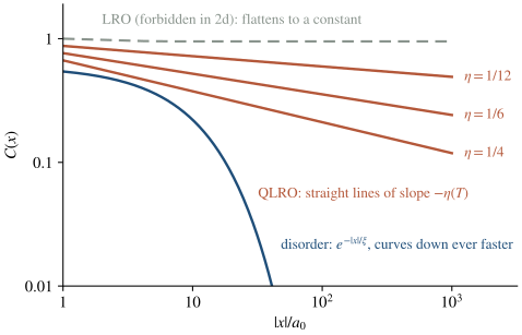
Figure 0. The three decay regimes on a log–log plot. QLRO is the odd one out in Landau’s world: an entire phase of straight lines whose slope is a continuous function of temperature. The QLRO lines are computed from the spin-wave correlator $C(x)=e^{-\kappa /\beta }|x{|}^{-\eta }$ of §3.4, with $\eta =1/2\pi \beta$, at $\eta =1/12$, $1/6$ and $1/4$; in the lattice model the exponent belongs to the renormalized stiffness (the physical picture below), so only the slopes carry over. The LRO and disordered curves are schematic.

Physical picture. The exponent grows with temperature — hotter means faster decay — and at the BKT point it takes the universal value $\eta (T_{BKT})=\frac{1}{4}$. Read that statement carefully: it is $\eta =1/2\pi {\beta }_R$ evaluated at the renormalized stiffness, which satisfies $\pi {\beta }_R=2$ exactly at the transition (Week 4); the bare critical coupling is model-dependent and larger, ${\beta }_c\approx 1.12$ for this cosine model [Stated — refs: Hasenbusch, J. Phys. A 38 (2005) 5869], because vortex pairs screen the stiffness downward before the transition is reached. The experiments test the equivalent statement about the stiffness. In superfluid helium-4 films, Bishop and Reppy (Phys. Rev. Lett. 40 (1978) 1727) measured the superfluid density with a torsional oscillator and found that it drops to zero at the transition from the universal value predicted by Nelson and Kosterlitz (Phys. Rev. Lett. 39 (1977) 1201); that jump is the statement $\pi {\beta }_R=2$, and through $\eta =1/2\pi {\beta }_R$ it is the statement $\eta =\frac{1}{4}$. Note the division of labor, which the exact duality of Week 3 will make into a theorem: spin waves control how correlators decay inside the QLRO phase; vortices decide where the phase ends.

3.5 Mermin–Wagner: no true order in 2d [Model proof.]

The absence of long-range order is not an artifact of the approximation. We prove it inside the spin-wave model — which, since Gaussian fluctuations are the least disordering fluctuations available, is the model-proof core of the general theorem.

Put the system in a finite box of linear size $L$ and ask for the magnetization $⟨e^{i{\theta }_x}⟩$ (fix the zero mode, e.g. ${\sum }_x{\theta }_x=0$, which is what a symmetry-breaking field would do). By the lemma of §3.2,

$$⟨e^{i{\theta }_x}⟩=e^{-\frac{1}{2}⟨{\theta }_x^2⟩},⟨{\theta }_x^2⟩=\frac{1}{\beta }\frac{1}{L^2}\sum _{k\ne 0}\frac{1}{{\hat{k}}^2}\stackrel{L\to \infty }{\to }\frac{1}{\beta }{\int }_{2\pi /L}^{\pi }\frac{d^{2}k}{(2\pi {)}^2}\frac{1}{k^2}+\text{finite}=\frac{1}{2\pi \beta }\ln \frac{L}{a_0}+\text{finite}.$$

The infrared sum diverges logarithmically with the box size. Thus

$$⟨e^{i{\theta }_x}⟩\sim (\frac{a_0}{L}{)}^{\frac{1}{4\pi \beta }}\stackrel{L\to \infty }{\to }0\text{for every }\beta <\infty .$$

The would-be order parameter dies — killed by the soft spin waves themselves, at any nonzero temperature. This is the content of the Mermin–Wagner theorem (Mermin & Wagner, Phys. Rev. Lett. 17 (1966) 1133; Hohenberg 1967): a continuous symmetry does not break spontaneously in $d\le 2$ at $T>0$. The general theorem upgrades the Gaussian estimate to an inequality (Bogoliubov) valid for the interacting model [Stated — refs]; the mechanism is exactly the one displayed. $\square$

The moral for this course: in 2d, the interesting transitions are between two disordered phases (power-law vs exponential decay), and no local order parameter can see them. This is the first of many times Landau’s toolbox comes up empty — the recurring predicament that Semester II resolves with generalized symmetries.

4. Vortices: the defects compactness forces

4.1 Definition and an explicit lattice vortex [Computed.]

A vortex of charge $q\in \mathbb{Z}$ is a configuration whose phase winds by $2\pi q$ around some plaquette: for every lattice loop $C$ encircling it once,

$$\sum _{\ell \in C}(d\theta {)}_{\ell }=2\pi q,$$

where each bond difference $(d\theta {)}_{\ell }={\theta }_y-{\theta }_x$ is reduced to the fundamental branch $(-\pi ,\pi ]$. Because θ is compact, this sum need not vanish; because it is a winding number, it is quantized and stable against any local smooth deformation.

Here is a charge-1 vortex, explicitly, centered on a plaquette (Figure 1). Assign to each site the polar angle of that site as seen from the plaquette center. On the four sites nearest the center the angles are $45°,135°,225°,315°$:

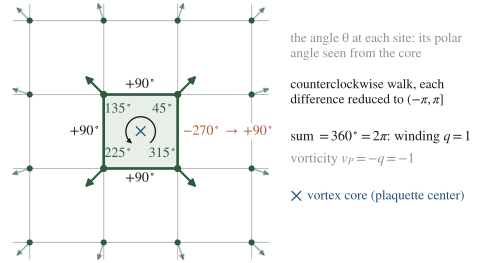
Figure 1. A charge-1 lattice vortex: site phases around the core plaquette, every spin computed from the polar-angle rule.

Walk the plaquette counterclockwise and take each difference in $(-\pi ,\pi ]$:

$$135°-45°=90°,225°-135°=90°,315°-225°=90°,45°-315°=-270°\stackrel{\mathrm{mod}360°}{\to }90°.$$

Sum: $360°=2\pi$. Winding number 1. On any plaquette not containing the core, the four branch-reduced differences sum to zero (each is small and the configuration is smooth there) — the vortex charge is localized on one plaquette. This “one integer per plaquette” bookkeeping is formalized in Week 2 (the vorticity is a 2-cochain; with the orientations of conventions §4 a counterclockwise $+2\pi$ winding has vorticity $v_P=-1$, so that $v_P=-q$) and is the variable the Week 3 duality sums over.

Note the branch reduction doing real work in the fourth bond: that step is the compactness. Unwrap θ to $\mathbb{R}$ and the sum telescopes to zero identically — which is how §3 lost the vortices.

4.2 Vortex energy [Computed.]

Far from the core the configuration is smooth and the spin-wave energy functional applies: $E=\frac{\beta }{2}\int d^{2}r|\nabla \theta {|}^2$ (lattice sums go over to integrals at distances $\gg a_0$). For the charge-$q$ vortex $\theta =q\phi$ (polar angle), so $|\nabla \theta |=q/r$ and

$$E_q=\frac{\beta }{2}{\int }_{a_0}^L(2\pi rdr)\frac{q^2}{r^2}=\pi \beta q^2\ln \frac{L}{a_0}+E_{\mathrm{core}}^{(q)},$$

with the core energy $E_{\mathrm{core}}$ collecting the lattice-scale region $r\lesssim a_0$ where the continuum estimate fails. Two features carry the whole subject:

• Logarithmic growth with system size $L$ — the marginal case. (In $d=3$ the same integral gives an energy per unit length of vortex line; the defect is a string with tension. In the gauge theories of Block C, the analogous integrals converge and the defects are finite-action instantons or worldlines — the table of Week 8.)
• Quadratic charge dependence $E\propto q^2$: two elementary vortices repel; a charge-2 vortex prefers to dissociate; only $q=\pm 1$ matters at low fugacity.

4.3 The pair, and the Coulomb analogy [Heuristic.]

A vortex–antivortex pair at separation $r$: superpose $\theta ={\phi }_{+}(x)-{\phi }_{-}(x)$ (polar angles about the two cores). Figure 2 draws this configuration on the lattice for $r=3$.

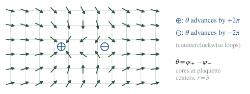
Figure 2. A vortex–antivortex pair, each arrow giving the spin direction θ at a site: on a counterclockwise loop θ advances by +2π around ⊕ and by −2π around ⊖, the spins between the cores point backwards, and far from the pair they return to alignment, so the gradient energy is confined to a region of size r.

At distances $\gg r$ the two windings cancel and $|\nabla \theta |$ decays as $r/|x{|}^2$ (a dipole field), so the energy integral is cut off at scale $r$ instead of $L$:

$$E_{\mathrm{pair}}(r)=2\pi \beta \ln \frac{r}{a_0}+2E_{\mathrm{core}}.$$

Finite, but growing logarithmically with separation: opposite vortices are logarithmically confined into dipoles. A logarithm is the 2d Coulomb potential, and two later derivations make the analogy exact and replace the cutoff argument: Week 3 §4 obtains the vortex sector of the Villain model as an exact neutral lattice Coulomb gas whose long-distance form is this pair energy, with $E_{\mathrm{core}}=2{\pi }^2\beta \kappa$ setting the fugacity, and Week 4 §2.2 evaluates the same field-energy integral by Green’s identity (the gradient of a polar angle is the gradient of $\ln |x|$ rotated by 90°), which gives $\int d^{2}x|\nabla \theta {|}^2=4\pi \ln (r/a_0)$. The phase transition is therefore a question about the electrostatics of that gas.

4.4 Why the spin-wave story cannot be complete [Heuristic — made exact in Weeks 3–4.]

The Gaussian phase of §3 assumed vortices away. But a single free vortex has finite free-energy cost $E_1=\pi \beta \ln (L/a_0)$ against an entropy $S_1=\ln (L/a_0{)}^2=2\ln (L/a_0)$ from its possible positions:

$$F_1=E_1-S_1=(\pi \beta -2)\ln \frac{L}{a_0}.$$

For $\beta >2/\pi$ the cost wins and free vortices are absent (only bound dipoles, harmless at long distance): QLRO survives. For $\beta <2/\pi$ entropy wins, vortices proliferate, and — as the plasma screens the angular rigidity — correlations decay exponentially. The crossing point $\pi \beta =2$ is the BKT estimate. Its precise status (Week 4): as a condition on the renormalized stiffness — the coefficient actually multiplying the vortex logarithm at long distance — it is exact, because the vortex operator is marginal there; as a prediction for the bare lattice coupling it is only an estimate, since the bound pairs themselves screen β downward before the transition. Monte Carlo places the bare critical coupling at ${\beta }_c\approx 1.12$ for the cosine model and ${\beta }_c\approx 0.75$ for the Villain model, both well above $2/\pi \approx 0.64$ [Stated — refs: Hasenbusch, J. Phys. A 38 (2005) 5869; Janke and Nather, Phys. Rev. B 48 (1993) 7419]. What this argument lacks — interactions among many vortices, screening, renormalization — is supplied by the exact duality (Week 3) and the RG (Week 4).

5. Tool I: the character expansion

The first of the two computational tools of the course, met in the cleanest place: the one-dimensional XY model (the O(2) rotor chain), exactly solvable, no vortices in the way. The same expansion powers the strong-coupling analysis of lattice gauge theory in Week 6, with characters of $SU(N)$ replacing $e^{in\theta }$.

5.1 Transfer matrix and Fourier diagonalization [Computed.]

For $N$ sites on a ring,

$$Z=\prod _{i=1}^N{\int }_{-\pi }^{\pi }\frac{d{\theta }_i}{2\pi }{e}^{\beta {\sum }_i\cos ({\theta }_i-{\theta }_{i+1})}=\mathrm{Tr}{T}^N,T(\theta ,{\theta }^{\prime })=e^{\beta \cos (\theta -{\theta }^{\prime })}.$$

The kernel depends only on $\theta -{\theta }^{\prime }$ — it commutes with rotations — so it is diagonalized by the characters $e^{in\theta }$ of $U(1)$. Expand the kernel in its Fourier series:

$$e^{\beta \cos \varphi }=\sum _{n=-\infty }^{\infty }{I}_n(\beta )e^{in\varphi },I_n(\beta )\equiv {\int }_{-\pi }^{\pi }\frac{d\varphi }{2\pi }{e}^{\beta \cos \varphi }{e}^{-in\varphi }.$$

The coefficient integral is precisely the standard integral representation of the modified Bessel function $I_n$ — that identification is the derivation of the Jacobi–Anger expansion; nothing is imported. Acting on a character:

$$(T{e}^{in\cdot })(\theta )=\int \frac{d{\theta }^{\prime }}{2\pi }{e}^{\beta \cos (\theta -{\theta }^{\prime })}{e}^{in{\theta }^{\prime }}=I_n(\beta )e^{in\theta }.$$

So the spectrum of $T$ is $\{I_n(\beta ){\}}_{n\in \mathbb{Z}}$, and

$$Z=\sum _{n\in \mathbb{Z}}{I}_n(\beta {)}^N,f=-\underset{N\to \infty }{\lim }\frac{1}{N}\ln Z=-\ln I_0(\beta ),$$

since $I_0(\beta )>I_1(\beta )>I_2(\beta )>\cdots >0$ for $\beta >0$. The integer $n$ — the character label — is a conserved “electric” quantum number flowing down the chain; it is the 1d shadow of the electric-flux variables that dominate Blocks B–C.

5.2 The correlator and its asymptotics [Computed.]

Insert charge operators and use the same diagonalization. With $0<r<N$,

$$⟨e^{i{\theta }_0}{e}^{-i{\theta }_r}⟩=\frac{1}{Z}\mathrm{Tr}\left(T^{N-r}{e}^{i\hat{\theta }}{T}^r{e}^{-i\hat{\theta }}\right).$$

Work in the character basis $|n⟩\leftrightarrow e^{in\theta }$, where $T|n⟩=I_n(\beta )|n⟩$ and the insertion operator acts as a charge raiser: $e^{i\theta }\cdot e^{in\theta }=e^{i(n+1)\theta }$, i.e. $e^{i\hat{\theta }}|n⟩=|n+1⟩$. The trace becomes a one-line sum:

$$\mathrm{Tr}\left(T^{N-r}{e}^{i\hat{\theta }}{T}^r{e}^{-i\hat{\theta }}\right)=\sum _{n\in \mathbb{Z}}{I}_n(\beta {)}^{N-r}{I}_{n+1}(\beta {)}^r$$

(the charge is raised to $n+1$ on the stretch of length $r$ between the insertions and returns to $n$ outside — charge conservation made diagrammatic). Dividing by $Z={\sum }_n{I}_n^N$, the $N\to \infty$ limit is dominated by $n=0$ in both sums:

$$⟨e^{i{\theta }_0}{e}^{-i{\theta }_r}⟩\stackrel{N\to \infty }{\to }(\frac{I_1(\beta )}{I_0(\beta )}{)}^r=e^{-r/\xi },\boxed{\xi (\beta )=[\ln \frac{I_0(\beta )}{I_1(\beta )}{]}^{-1}.}$$

Both limits, derived. Small β: from the integral representation, $I_n(\beta )=\frac{1}{n!}\left(\frac{\beta }{2}{)}^n\right(1+O({\beta }^2))$ (expand $e^{\beta \cos \varphi }$ and pick the term with net charge $n$), so

$$\frac{I_1}{I_0}\simeq \frac{\beta }{2},\xi \simeq \frac{1}{\ln (2/\beta )}\to 0:$$

strong disorder, correlation length below one lattice spacing. Large β: saddle point of the coefficient integral at $\varphi =0$ — expand $\cos \varphi \simeq 1-{\varphi }^2/2$, extend the range, and keep the Gaussian correction:

$$I_n(\beta )=\frac{e^{\beta }}{\sqrt{2\pi \beta }}(1-\frac{4n^2-1}{8\beta }+O({\beta }^{-2}))⟹\frac{I_1}{I_0}\simeq 1-\frac{1}{2\beta },\xi \simeq 2\beta .$$

The correlation length grows only linearly in β: no phase transition at any finite temperature in 1d, as expected — there is not enough room in one dimension for the ordering tendency to win. The 2d miracle (a transition without symmetry breaking) needs the marginal vortex logarithm, which 1d does not have.

Physical picture. The character expansion converts an integral over a compact group into a sum over its irreducible representations — from “field space” to “charge space.” That is the move that will turn Wilson’s plaquette integrals into flux-tiling combinatorics in Week 6: there, the statement “a link integrates to zero unless its charges cancel” becomes the geometric statement “Wilson loops must be tiled by surfaces,” and the area law falls out. Learn the 1d version cold; the gauge version is the same manipulation wearing group theory.

6. Tool II: Poisson resummation — winding versus momentum

The second tool is an identity between two ways of summing over the integers:

$$\boxed{\sum _{n\in \mathbb{Z}}f(n)=\sum _{w\in \mathbb{Z}}{\int }_{-\infty }^{\infty }dxf(x)e^{2\pi iwx}}$$

(Poisson resummation; proved as a two-line Fourier-series statement in Week 2 §7, used freely afterward). It trades a sum over “momenta” $n$ for a sum over “windings” $w$, exchanging small and large coupling. Rather than cite it, this section derives its physical content in the cleanest quantum-mechanical setting, by the method of images — so that the identity arrives with a mechanism attached.

6.1 A particle on a ring, two ways [Computed.]

Free particle on a circle of circumference $2\pi$, moment of inertia β, Euclidean time interval $\mathcal{T}$.

Momentum (spectral) representation. Angular momentum is quantized, $\hat{L}=-i{\partial }_{\theta }$ with eigenvalues $n\in \mathbb{Z}$ and energies $E_n=n^2/2\beta$:

$$Z=\mathrm{Tr}{e}^{-\mathcal{T}\hat{H}}=\sum _{n\in \mathbb{Z}}{e}^{-\mathcal{T}{n}^2/2\beta }.$$

Winding (path-integral) representation, via images. The Euclidean propagator on the line is the heat kernel

$$K_{\mathbb{R}}(\theta ,{\theta }^{\prime };\mathcal{T})=\sqrt{\frac{\beta }{2\pi \mathcal{T}}}{e}^{-\beta (\theta -{\theta }^{\prime }{)}^2/2\mathcal{T}}.$$

The propagator on the circle must satisfy the same heat equation and be $2\pi$-periodic in both arguments; by uniqueness of heat-equation solutions with given initial data, it is the periodization of the line kernel — the sum over image points:

$$K_{S^1}(\theta ,{\theta }^{\prime };\mathcal{T})=\sum _{w\in \mathbb{Z}}{K}_{\mathbb{R}}(\theta ,{\theta }^{\prime }+2\pi w;\mathcal{T}).$$

Each image term is the contribution of paths that wind $w$ times. Tracing:

$$Z={\int }_0^{2\pi }d\theta K_{S^1}(\theta ,\theta ;\mathcal{T})=2\pi \sqrt{\frac{\beta }{2\pi \mathcal{T}}}\sum _{w\in \mathbb{Z}}{e}^{-\beta (2\pi w{)}^2/2\mathcal{T}}=\sqrt{\frac{2\pi \beta }{\mathcal{T}}}\sum _{w\in \mathbb{Z}}{e}^{-2{\pi }^2\beta w^2/\mathcal{T}}.$$

The two expressions are equal — same trace, computed in two bases — and their equality

$$\sum _n{e}^{-\mathcal{T}{n}^2/2\beta }=\sqrt{\frac{2\pi \beta }{\mathcal{T}}}\sum _w{e}^{-2{\pi }^2\beta w^2/\mathcal{T}}$$

is precisely the Poisson identity for a Gaussian (the Jacobi theta transformation), here derived rather than invoked, with the prefactor produced automatically. Note the coupling inversion: the momentum sum converges fast when $\mathcal{T}/\beta$ is large, the winding sum when it is small. One partition function, two asymptotic regimes, each with its natural variable.

Physical picture. Winding and momentum are Poisson-dual: the configuration that wraps the target circle (a soliton, a vortex, a flux line — depending on dimension) is, in the dual description, a highly excited state of the tower of charges. This is the seed of every duality in the course. In Week 3 the vortices of the XY model emerge as the Poisson dual of its spin waves; in Week 8 the magnetic monopoles of compact electrodynamics emerge as the Poisson dual of its electric fluxes. The method-of-images derivation supplies the mechanism to remember: dualizing = re-organizing the same sum by which topological sector the paths belong to.

6.2 The Villain preview

The ring computation was exact because the action was Gaussian within each winding sector. The XY cosine is not — but nothing stops us from replacing it with a function that is: keep the $2\pi$-periodicity, make each branch Gaussian,

$$e^{\beta \cos \varphi }⟶V_{\beta }(\varphi )=\sum _{n\in \mathbb{Z}}{e}^{-\frac{\beta }{2}(\varphi -2\pi n{)}^2}.$$

This is the Villain action. Its character coefficients follow in one line, because the sum over branches unfolds the period integral into an integral over the whole line (branch $n$ contributes the interval shifted by $2\pi n$, and $e^{-im\varphi }$ is $2\pi$-periodic):

$${\tilde{V}}_m\equiv {\int }_{-\pi }^{\pi }\frac{d\varphi }{2\pi }{V}_{\beta }(\varphi )e^{-im\varphi }={\int }_{-\infty }^{\infty }\frac{d\varphi }{2\pi }{e}^{-\frac{\beta }{2}{\varphi }^2-im\varphi }=\frac{e^{-m^2/2\beta }}{\sqrt{2\pi \beta }},$$

where the last step completes the square as in §3.2. That is, $V_{\beta }(\varphi )=(2\pi \beta {)}^{-1/2}{\sum }_{m\in \mathbb{Z}}{e}^{-m^2/2\beta +im\varphi }$, the periodic-Gaussian identity of conventions §3. These exact Gaussians are to be compared with the Bessel coefficients $I_m(\beta )$ of the cosine; the two agree to leading order at large β and share all universal physics, and Problem 5 makes the comparison quantitative. On the Villain form, the manipulation of §6.1 (organize the sum by topological sector, then resum) goes through exactly in any dimension. Executing it for the 2d XY model is Week 3, and the outcome is the vortex Coulomb gas promised in §4.

7. Historical note

The theory of the 2d XY transition was built twice. Berezinskii (1971, JETP) identified the low-temperature phase’s power-law order and the role of vortex unbinding; Kosterlitz and Thouless (1973), independently, gave the energy–entropy argument of §4.4 and, with Kosterlitz’s 1974 RG, the flow equations and the universal predictions (Week 4). Mermin–Wagner (1966) predates both and set the puzzle: if 2d systems with continuous symmetry cannot order, what is the helium film’s observed transition into? The answer — a phase transition between two disordered phases, driven by topological defects, with no local order parameter — was genuinely new physics, and it is the prototype for everything in this course: Wegner’s transition (Week 5), Polyakov’s confinement (Weeks 9–10), and topological order (Semester II) are all “BKT-type” in this structural sense.

8. Subtleties and fine print

F1 — Mermin–Wagner forbids order, not transitions. The theorem kills $⟨\vec{S}⟩$, nothing else. Phase transitions diagnosed by non-local quantities (stiffness jumps, defect-fugacity relevance, asymptotics of correlators) are untouched. The BKT transition lives entirely in observables Mermin–Wagner does not constrain. Keep the logical shape: “no local order parameter” never implies “no phase structure” — the course’s recurring theme.

F2 — η’s normalization is cutoff-dependent; η’s value at the transition is not. The amplitude $e^{-\kappa /\beta }$ of the correlator $C(x)$ depends on the lattice constant κ — microscopic, non-universal. The exponent $\eta (\beta )=1/2\pi \beta$ depends on β, which itself renormalizes (Week 4); what is universal is the exponent expressed through the renormalized stiffness, and in particular $\eta =1/4$ exactly at $T_{BKT}$. Distinguish always: amplitudes non-universal, exponents-at-criticality universal.

F3 — Winding is conserved; windings still disappear pairwise. Vortex charge on a large contour is a homotopy invariant, but nothing prevents a vortex–antivortex pair from nucleating or annihilating locally inside it. Charge conservation constrains the total, not the population. This is why fugacity (pair-creation cost, set by $E_{\mathrm{core}}$) — not any conservation law — controls the vortex density.

F4 — Villain vs cosine is a choice of core, already visible in 1d. The two transfer matrices have character coefficients $e^{-m^2/2\tilde{\beta }}$ (Villain) vs $I_m(\beta )/I_0(\beta )$ (cosine). Matching the $m=1$ coefficients defines $\tilde{\beta }(\beta )$; the residual mismatch at $m\ge 2$ is algebraically small in $1/\beta$, first appearing at order ${\beta }^{-3}$ (Problem 5(c)), and renormalizes only the vortex core energy and multi-charge fugacities in 2d. Universal content (exponents, the jump, $T_{BKT}$‘s existence) is form-independent; non-universal content ($T_{BKT}$‘s numerical value, amplitudes) is not. Problem 5 makes this quantitative.

F5 — Only differences of the Green function exist in 2d. $G(x)$ alone is IR-divergent; every physical quantity assembled this week ($⟨({\theta }_x-{\theta }_0{)}^2⟩$, pair energies) involves $a(x)=G(0)-G(x)$, which is finite. On a finite torus the divergence appears as the $k=0$ zero mode, which must be omitted or fixed — the same zero mode that, in Week 3, enforces exact vortex-charge neutrality on the Coulomb gas. The IR pathology of 2d is not a nuisance; it is a constraint generator.

F6 — The branch choice in $(d\theta {)}_{\ell }$ is physics, not bookkeeping. Defining bond differences in $(-\pi ,\pi ]$ is what localizes vortex charge on plaquettes (§4.1). A different branch convention shifts which plaquette carries the core but never the total winding on large loops — a “lattice gauge choice” for defects, formalized by the integer field $n_{\ell }$ of the Villain form in Week 3.

9. Common misconceptions

• “Mermin–Wagner says nothing happens in 2d.” Wrong; see F1. It says the symmetry-breaking scenario is unavailable. The helium film transition is real, measured, and BKT.
• “η is the critical exponent of the XY model.” η is a function $\eta (T)=1/2\pi {\beta }_R(T)$ along a line of fixed points; only its endpoint value $\eta (T_{BKT})=1/4$ is a single universal number. Quoting “η of the 2d XY model” without a temperature is meaningless.
• “Compactness is a choice of description that physics cannot feel.” The spectrum of charges ($e^{in\theta }$, $n\in \mathbb{Z}$), the existence of vortices, and ultimately the entire phase diagram follow from the identification $\theta \sim \theta +2\pi$. Decompactify and all of it disappears (§3’s Gaussian model is exactly that theory: forever critical, no transition).
• “A charge-2 vortex is just a bigger vortex.” It costs $4\times$ the energy of a charge-1 vortex but gains no extra positional entropy; it is unstable to dissociation into two unit vortices. Only $|q|=1$ matters near the transition.

10. What to take away

1. Compactness is topological data. ${\pi }_1(U(1))=\mathbb{Z}$ forces quantized charges ($e^{in\theta }$) and quantized defects (vortices). The “real scalar” of a first course is the decompactified — and physically different — theory.
2. Spin waves give QLRO, and kill LRO. The Gaussian sector produces power-law correlations with $\eta =1/2\pi \beta$ [Computed; the constant κ of the amplitude $e^{-\kappa /\beta }$ is quoted, Stated — refs], and its own IR fluctuations prove Mermin–Wagner in the model case [Model proof]: 2d transitions must be order-parameter-free.
3. Vortices are logarithmically confined Coulomb charges. $E_q=\pi \beta q^2\ln (L/a_0)$, pairs cost $2\pi \beta \ln r$; the energy–entropy balance flags $\pi \beta =2$ as the marginality condition — exact for the renormalized stiffness, an estimate for the bare coupling. The core constant κ of the lattice Green function will become the fugacity of Week 3’s Coulomb gas.
4. Two tools, exact and reusable. The character expansion (compact integral → charge sum; the strong-coupling engine of Week 6) and Poisson resummation (momentum sum ↔ winding sum, derived here by the method of images; the duality engine of Weeks 3, 8, and Semester II).

11. Looking ahead: Week 2

Before the vortices of the full 2d model can be resummed, we need the language that says where fields and defects live — sites, links, plaquettes, and their dual lattice — and that converts “topology” into finite linear algebra. Week 2 builds it: chains and cochains, the boundary and coboundary operators, the homology of the torus computed by hand (matrices included), Poincaré duality, and the intersection pairing whose single “+1” on the torus later becomes the clock–shift algebra of topological order. With that toolkit, Week 3 performs the XY → Coulomb-gas duality with every constant tracked.

12. Problem set

Problems 1–4 are the classroom core and are solvable from the note alone; Problems 5⋆ and 6⋆ are self-study consolidation, each with a hint or an indicated method; Problem 7⋆⋆ is a research extension that states what is known, what is explored, the source it needs and what counts as completion.

Core problems (everyone).

1. Rotor chain thermodynamics. From $Z={\sum }_n{I}_n(\beta {)}^N$: (a) derive the internal energy per site $u(\beta )=-I_1(\beta )/I_0(\beta )$ and the entropy in both temperature limits; (b) using the asymptotics derived in §5.2, show the specific heat is smooth for all β — no transition — and locate its maximum numerically to two digits.

2. Finite-size scaling of the magnetization. In the spin-wave model on an $L\times L$ torus with the zero mode fixed, refine §3.5: compute the subleading (constant) term in $⟨{\theta }_x^2⟩$ and show $⟨e^{i\theta }⟩=c(a_0/L{)}^{1/4\pi \beta }(1+O(1/L^2))$. How would you extract $\eta (\beta )$ from magnetization data on finite lattices?

3. Higher-charge correlators. Show that $⟨e^{iq({\theta }_x-{\theta }_0)}⟩$ decays as $|x{|}^{-q^2\eta (\beta )}$ in the spin-wave model, and verify that its amplitude is $e^{-q^2\kappa /\beta }$. Why does the $q^2$ in the exponent mirror the $q^2$ in the vortex energy (§4.2)? (The two are Poisson-dual statements; Week 3 makes this precise.)

4. Dipole gas at low temperature. Treat the vortex sector below $T_{BKT}$ as a dilute gas of $\pm$ pairs with the §4.3 energy and fugacity $y=e^{-E_{\mathrm{core}}}$ per vortex. (a) Compute the mean-square dipole size $⟨r^2⟩={\int }_{a_0}^{\infty }{r}^{2}rdr{r}^{-2\pi \beta }/{\int }_{a_0}^{\infty }rdr{r}^{-2\pi \beta }$ and find at which β it first diverges. (b) Show that this divergence occurs exactly at the energy–entropy point $\pi \beta =2$ of §4.4, so that the two criteria coincide, and say what each one measures: part (a) the size of the bound pairs, §4.4 the free energy of a single free vortex. (Cut the numerator of (a) off at a radius $R$ and compare its growth with the single-vortex weight $e^{-F_1}$ in a box of size $R$.) (c) The bound pairs screen the stiffness; Week 4 §2.2 derives ${\beta }_R^{-1}={\beta }^{-1}+4{\pi }^3{y}^2{\int }_{a_0}^{\infty }\frac{dr}{a_0}(\frac{r}{a_0}{)}^{3-2\pi \beta }+O(y^4)$, whose integral is, up to powers of $a_0$, the numerator of (a). Use this to explain why the transition, which sits at $\pi {\beta }_R=2$, is reached at a bare coupling above $2/\pi$, as the Monte Carlo values ${\beta }_c\approx 1.12$ (cosine) and ${\beta }_c\approx 0.75$ (Villain) quoted in §4.4 show.

Starred problems (Ph.D. expected; ambitious M.Sc. encouraged).

5⋆. Villain vs cosine, quantitatively. (a) With the coefficients ${\tilde{V}}_m$ of §6.2, repeat §§5.1–5.2 for the Villain chain: show that the transfer-matrix spectrum is $\{{\tilde{V}}_m{\}}_{m\in \mathbb{Z}}$ and that $⟨e^{i{\theta }_0}{e}^{-i{\theta }_r}⟩\to e^{-r/2\beta }$, so that $\xi =2\beta$ exactly at every β, and compare with the cosine chain, whose ξ approaches $2\beta$ only at large β. (b) Define the effective Villain coupling by matching $m=1$ coefficients, $e^{-1/2\tilde{\beta }}=I_1(\beta )/I_0(\beta )$, and expand $\tilde{\beta }(\beta )$ at large and small β (use the small-β form of §5.2 and, at large β, the series quoted in (c)). (c) Carry the large-β expansion of §5.2 to third order with the asymptotic series

$$I_m(\beta )\simeq \frac{e^{\beta }}{\sqrt{2\pi \beta }}\sum _{k\ge 0}\frac{(-1{)}^k}{k!(8\beta {)}^k}\prod _{j=1}^k(4m^2-(2j-1{)}^2),$$

whose $k=1$ term is the correction displayed in §5.2, and show that

$$\ln \frac{I_m(\beta )}{I_0(\beta )}=-\frac{m^2}{2\beta }-\frac{m^2}{4{\beta }^2}+\frac{1}{{\beta }^3}(\frac{m^4}{24}-\frac{13m^2}{48})+O({\beta }^{-4}).$$

Conclude that the $m=1$ matching of (b) absorbs every term through $O({\beta }^{-2})$, where the dependence on $m$ is purely $m^2$, and that the first order a single rescaled Villain coupling cannot match is ${\beta }^{-3}$, with residual $m^2(m^2-1)/24{\beta }^3$ (for $m=2$, $1/2{\beta }^3$): algebraic in $1/\beta$, not exponentially small. Argue that it only shifts the vortex core energy and the multi-charge fugacities in 2d. (Hint: in the current representation of Week 3 §2 the character coefficients are the link weights of the conserved integer currents, so the residual reweights only links that carry $|m|\ge 2$.) (Fine print F4 made quantitative.)

6⋆. Twisted boundary conditions and the stiffness. Impose ${\theta }_{x+L_1\hat{1}}={\theta }_x+\alpha$ on the 2d spin-wave model on an $L_1\times L_2$ torus. (a) Write ${\theta }_x=\alpha x_1/L_1+{\varphi }_x$ with φ periodic, show that the cross term vanishes by periodicity, and conclude that at the Gaussian (spin-wave) level the twist free energy is exactly

$$\Delta F(\alpha )=-\ln \frac{Z(\alpha )}{Z(0)}=\frac{\beta {\alpha }^2}{2}\frac{L_2}{L_1},$$

with no higher powers of α. Writing $\Delta F=\frac{{\rm Y}}{2}{\alpha }^2{L}_2/L_1$ defines the helicity modulus (spin stiffness), and the spin-wave model has ${\rm Y}=\beta$. (b) Explain why vortices can reduce ${\rm Y}$ but spin waves cannot, and why ${\rm Y}$ is therefore the natural non-local order parameter for BKT (the quantity whose universal jump Week 4 derives). (Hint: in (a) the integral over φ does not depend on α; a bound vortex pair polarizes in the uniform phase gradient $\alpha /L_1$ and partly cancels it, which is the screening of Week 4 §2.2.) (c) Connect $\alpha$ to a background field for the $U(1)$ symmetry, the first and simplest instance of “coupling a symmetry to a background”, the systematic subject of Semester II. (Hint: the substitution of (a) moves the twist from the boundary condition into the action, where every 1-link carries $({\varphi }_{x+\hat{1}}-{\varphi }_x+\alpha /L_1{)}^2$; that is $(d\varphi +A{)}^2$ with the constant link field $A_1=\alpha /L_1$, whose holonomy around the torus is α.)

⋆⋆ problems (research extension; optional).

7⋆⋆ (optional, harder). The lattice constant κ. What is known. The subtracted Green function $a(x)=G(0)-G(x)$ of §3.3 is known exactly on the square lattice (Spitzer, Principles of Random Walk, §15, whose potential kernel of simple random walk is $4a(x)$ in our normalization): $a(1,0)=\frac{1}{4}$, $a(1,1)=1/\pi$, and $a(x)=\frac{1}{2\pi }\ln |x|+\kappa +O(|x{|}^{-2})$ at large distance, with $\kappa =(2{\gamma }_E+\ln 8)/4\pi =0.257343\dots$ What is explored. How much of this follows from the lattice alone, and how fast the asymptotic form sets in. (a) Show that $\Delta G=\delta$ at $x=0$, together with the fourfold lattice symmetry, gives $a(1,0)=\frac{1}{4}$, and that the same equation at $x=(1,0)$ gives only $a(2,0)+2a(1,1)=1$: symmetry fixes one combination of the next two values and no more. (b) Obtain $a(1,1)=1/\pi$, and therefore $a(2,0)=1-2/\pi$, from the Fourier integral of §3.3 (rotate the momentum axes by 45°, $u=\frac{k_1+k_2}{2}$, $v=\frac{k_1-k_2}{2}$, and use ${\int }_{-\pi }^{\pi }\frac{dv}{2\pi }\frac{1}{1-c\cos v}=(1-c^2{)}^{-1/2}$ for $|c|<1$). (c) Evaluate the momentum integral numerically along the lattice axis and the diagonal, verify κ to three digits, and measure how the deviation from the asymptotic form decays with $|x|$. Completion: the derivations of (a) and (b); a table of $a(x)-\frac{1}{2\pi }\ln |x|-\kappa$ at $|x|=1,\sqrt{2},2$ and at a few larger separations in both directions; κ to three digits with an error estimate; and a statement, supported by the table, of how the $O(|x{|}^{-2})$ correction depends on the direction of $x$.

Self-study answer checkpoints

These checkpoints cover the core problems; starred and ⋆⋆ problems remain source-led.

1. Rotor chain. Since $I_0(\beta )>I_n(\beta )>0$ for $n\ne 0$, $\ln Z=N\ln I_0+\ln [1+{\sum }_{n\ne 0}(I_n/I_0{)}^N]$ and the bracket tends to 1, so $\ln Z/N\to \ln I_0(\beta )$ and $u=-{\partial }_{\beta }\ln I_0=-I_1/I_0$, using $I_0^{\prime }=I_1$. The entropy per site is $s=\ln I_0-\beta I_1/I_0$, with $s\simeq -{\beta }^2/4$ at high temperature and $s\simeq \frac{1}{2}-\frac{1}{2}\ln (2\pi \beta )$ at low temperature. With $I_1^{\prime }=I_0-I_1/\beta$ the specific heat is $$c={\beta }^2{\partial }_{\beta }\frac{I_1}{I_0}={\beta }^2[1-\frac{I_1}{\beta I_0}-(\frac{I_1}{I_0}{)}^2],$$ which grows as ${\beta }^2/2$ at small β, tends to the equipartition value $\frac{1}{2}$ from above at large β, and is analytic at every $\beta >0$ because $\ln I_0$ is. Its maximum is $c_{\max }\simeq 0.68$ at $\beta \simeq 2.5$ ($T\simeq 0.40J$). Common failure mode: expecting $s\to 0$ and $c\to 0$ at low temperature, or reading the maximum as a transition; for classical rotors $s\to -\infty$ logarithmically, $c\to \frac{1}{2}$, and the maximum is a smooth crossover.
2. Finite-size magnetization. With the zero mode fixed, $⟨{\theta }_x^2⟩={\beta }^{-1}{L}^{-2}{\sum }_{k\ne 0}{\hat{k}}^{-2}$ over $k=2\pi n/L$, and the decisive step is to separate the logarithm from the constant, $L^{-2}{\sum }_{k\ne 0}{\hat{k}}^{-2}=\frac{1}{2\pi }\ln L+c_1+O(L^{-2})$. Evaluating the sum for $L=8,\dots ,2048$ gives $c_1=0.04877$, with $(c_1(L)-c_1)L^2\to -0.029$; the closed form $c_1=\kappa -\frac{1}{2\pi }\ln \frac{\Gamma (1/4{)}^2}{2\sqrt{\pi }}$ follows from the continuum torus Green function. Therefore $$⟨e^{i\theta }⟩=e^{-c_1/2\beta }{L}^{-1/4\pi \beta }(1+O(L^{-2})),$$ so $c=e^{-c_1/2\beta }$, and η is minus twice the slope of $\ln ⟨|m|⟩$ against $\ln L$ at fixed β, where $m=L^{-2}{\sum }_x{e}^{i{\theta }_x}$. Common failure mode: taking the slope itself as η; the magnetization exponent is $1/4\pi \beta =\eta /2$, since $⟨|m|{⟩}^2$ scales as $C(L)\sim L^{-\eta }$.
3. Higher-charge correlators. The lemma of §3.2 with $A=q({\theta }_x-{\theta }_0)$ and $⟨A^2⟩=q^2\cdot \frac{2}{\beta }a(x)$ gives $$⟨e^{iq({\theta }_x-{\theta }_0)}⟩=e^{-q^{2}a(x)/\beta }=e^{-q^2\kappa /\beta }|x{|}^{-q^2/2\pi \beta },$$ that is, exponent $q^2\eta$ and amplitude $e^{-q^2\kappa /\beta }$. Both factors of $q^2$ come from the same quadratic action: a charge $q$ enters through $q^{2}a(x)/\beta$, a winding $q$ through $\pi \beta q^2\ln (L/a_0)$. The pair weight $r^{-2\pi \beta q^2}$ and the correlator $r^{-q^2/2\pi \beta }$ are exchanged by $\beta \to 1/4{\pi }^2\beta$, which is the duality of Week 3; in the language of conventions §5, it exchanges the scaling dimension $q^2/4\pi \beta$ of $e^{iq\theta }$ with the dimension $\pi \beta q^2$ of the charge-$q$ vortex. Common failure mode: dropping the factor 2 in $⟨({\theta }_x-{\theta }_0{)}^2⟩=2a(x)/\beta$, which gives the wrong exponent $q^2/4\pi \beta$ and the wrong amplitude $e^{-q^2\kappa /2\beta }$.
4. Dipole gas. The numerator converges only for $2\pi \beta >4$ and the denominator for $2\pi \beta >2$; for $\pi \beta >2$, $$⟨r^2⟩=a_0^2\frac{\pi \beta -1}{\pi \beta -2},$$ which diverges as $\beta \to 2/\pi$ from above, exactly where $F_1=(\pi \beta -2)\ln (L/a_0)$ changes sign. Cut at $R$, the numerator grows as $R^{4-2\pi \beta }=(R^{2-\pi \beta }{)}^2$, the square of the single-vortex weight $e^{-F_1}$ in a box of size $R$: pairs as large as the system are free vortices, which is why the two criteria coincide. Part (a) measures the size of the bound pairs, and therefore their polarizability, from inside the dipole phase; §4.4 measures the free energy of one free vortex, that is, the stability of the phase. For (c), ${\beta }_R<\beta$ at any $y>0$, so $\pi {\beta }_R=2$ requires $\pi {\beta }_c>2$; the correction is the integral of (a), which diverges at the naive point, so screening grows without bound as $2/\pi$ is approached from above, and a self-consistent treatment (the RG of Week 4) is needed to locate ${\beta }_c$. Common failure mode: dropping the measure $rdr$, which moves the divergence to $\beta =3/2\pi$, or reading the divergence of the denominator at $\beta =1/\pi$ as the transition.

---

Notes prepared for the generalized-symmetries course, Semester I Block A. Rewritten to the note-quality-template standard on 2026-07-10 (first draft 2026-07-01). Last revised 2026-09-28.