Week 4 — BKT, Kramers–Wannier, and the First Disorder Operators

Two stories close Block A, and they are secretly one. First: the Coulomb gas built in Week 3 ionizes — the Berezinskii–Kosterlitz–Thouless transition — and its renormalization group yields two predictions no Landau theory could produce: a universal jump in the stiffness and an essential singularity in the correlation length. Second: the 2d Ising model equals itself at the dual temperature — Kramers–Wannier — and the operator implementing the equality, the Kadanoff–Ceva disorder operator, is our first symmetry object living on an extended seam. Block A ends with the sentence the whole course elaborates: a duality is a statement about a wall.

How to use this chapter

• In class: in the first lecture derive the fugacity flow (§2.1), then the screening constant $4{\pi }^3$ with its field-energy integral (§2.2), and integrate the linearized flow to the invariant $C$, the separatrices, the universal jump and ${\ell }^{\ast }=\pi /\sqrt{bt}$ (§2.3, Figure 1); Problems 1 and 2 belong to this lecture. In the second, do the two Ising expansions and the self-dual point (§§3.1–3.3, Figure 2), then the seam weights and $⟨\mu \mu {⟩}_{\beta }=⟨\sigma \sigma {⟩}_{{\beta }^{\ast }}$ (§§4.1–4.2, Figure 3), with Problems 3 and 4.
• For self-study: the boundary-condition sectors of §3.4, the order–disorder algebra and the Jordan–Wigner fermion of §4.3, and the defect preview of §4.4. The one calculation to do alone is the sector formula of §3.4 with its prefactor $[2{\sinh }^{N}2\beta {]}^{-1}$, checked by enumerating all four sectors on both sides of the $2\times 3$ torus, the smallest torus on which the placement of the indices shows.
• Instructor checkpoint: $\pi \beta =2$ is exact for the renormalized stiffness ${\beta }_R$ and only an estimate for the bare coupling, whose critical values are ${\beta }_c\approx 1.12$ (cosine model) and ${\beta }_c\approx 0.75$ (Villain model), both above $2/\pi$ (§1(b)). And a twist α enters the tilt sectors of Week 3 as the phase $e^{i\alpha w_1}$, which gives ${\rm Y}=\beta$ at the Gaussian level; treated as a shift $w_1\to w_1+\alpha /2\pi$ it would give an exponentially small stiffness (Problem 2).

0. Reading

Primary: Kosterlitz & Thouless, J. Phys. C 6 (1973) 1181; Kosterlitz, J. Phys. C 7 (1974) 1046 (the RG). Kramers & Wannier, Phys. Rev. 60 (1941) 252. Kadanoff & Ceva, Phys. Rev. B 3 (1971) 3918.

Secondary:

• Kardar, Statistical Physics of Fields, ch. 8, the sections on topological defects in the XY model and on the renormalization group for the Coulomb gas: the RG derivation in conventions matching ours.
• Nelson & Kosterlitz, Phys. Rev. Lett. 39 (1977) 1201 — the universal jump; Bishop & Reppy, Phys. Rev. Lett. 40 (1978) 1727 — its measurement.
• Fradkin, Field Theories of Condensed Matter Physics, 2nd ed., ch. 3 — order/disorder operators in the language Semester II uses.

Proof-status labels as in Week 1. Inputs from Week 3: the Coulomb gas with (long-distance) fugacity $y=e^{-2{\pi }^2\beta \kappa }$, and the vortex-operator dimension ${\Delta }_{\mathrm{vortex}}=\pi \beta$.

1. The energy–entropy argument, sharpened [Heuristic.]

Week 1 §4.4 balanced one vortex’s energy against its positional entropy:

$$F_1=E_1-S_1=(\pi \beta -2)\ln \frac{L}{a_0},$$

sign change at $\beta =2/\pi$. Three sharpenings come before the RG of §2, which is the controlled treatment:

(a) Higher charges never win first. A charge-$q$ vortex has $F_q=(\pi \beta q^2-2)\ln (L/a_0)$: the unbinding threshold ${\beta }_q=2/\pi q^2$ sits at lower β (higher temperature) for larger $q$ — by the time charge-2 vortices would unbind, charge-1 vortices have long since proliferated and screened everything. Only $|q|=1$ matters. (Same conclusion from operator dimensions: ${\Delta }_q=\pi \beta q^2$, so $e^{2i\chi }$ is strongly irrelevant where $e^{i\chi }$ is marginal — Week 3, F6.)

(b) What the estimate gets exactly right — and what it does not. The argument balances the vortex energy against entropy using the unscreened stiffness, so the number it produces, “transition at $\pi \beta =2$,” is a statement about whichever stiffness actually multiplies the vortex logarithm at long distances. That is the renormalized stiffness ${\beta }_R$ — reduced below the bare β by the bound pairs themselves (§2). The exact, universal statement is therefore

$$\pi {\beta }_R(T_{BKT})=2,$$

the fixed-point condition of the RG below, while the bare critical coupling is model-dependent and sits above $2/\pi \approx 0.64$: Monte Carlo gives ${\beta }_c\approx 1.12$ for the cosine XY model (Hasenbusch, J. Phys. A 38 (2005) 5869) and ${\beta }_c\approx 0.75$ for the Villain model (Janke and Nather, Phys. Rev. B 48 (1993) 7419) [Stated — refs.]. Conflating the two is the single most common error in this subject; every "${\beta }_{BKT}=2/\pi$" in Weeks 1 and 3 is to be read as the marginality condition on the running stiffness, exact for ${\beta }_R$, heuristic for the bare coupling.

(c) What the argument cannot give. How the transition is approached (the flow), what is universal (the jump), the shape of $\xi (T)$ (essential singularity) — for these, renormalize.

Physical picture. In a helium film, “a free vortex” is not an abstraction: it is a mobile hole in the condensate that can be dragged by a flow, and a single one moving across the film dissipates supercurrent. Below $T_{BKT}$, every vortex is chained to a partner and the pair moves without net phase slip: the film flows forever. The transition is, operationally, the onset of free phase-slip carriers — which is why the experimental signature is a jump in the dissipationless stiffness and a sudden onset of broadband dissipation, both seen in the torsional-oscillator data. Energy–entropy is deciding whether a phase-slip carrier can afford to leave home.

2. The Kosterlitz renormalization group

The physics: at low temperature the plasma consists of bound $\pm$ dipoles. A dipole of size $r$ is polarizable; a gas of polarizable dipoles is a dielectric; a dielectric screens the interaction between widely separated charges. So the effective stiffness measured at scale $r$, call it ${\beta }_R(r)$, decreases as more dipole sizes are integrated in — and the fugacity of larger pairs is in turn controlled by the screened stiffness. Two coupled flows.

2.1 The fugacity flow, derived [Computed.]

From Week 3 §6, the vortex insertion $e^{\pm i\chi }$ is a scaling operator of dimension $\Delta =\pi {\beta }_R$: its two-point function decays as $r^{-2\pi {\beta }_R}$. The fugacity term in the sine-Gordon action is $2y{\sum }_{\tilde{x}}\cos \chi \to 2y\int \frac{d^{2}x}{a^2}\cos \chi$. Rescale the cutoff $a\to a{e}^{\ell }$: the measure contributes $e^{2\ell }$, the operator’s amplitude renormalizes as $e^{-\Delta \ell }$, so $y(\ell )=y{e}^{(2-\pi {\beta }_R)\ell }$, i.e.

$$\boxed{\frac{dy}{d\ell }=(2-\pi {\beta }_R)y+O(y^3).}$$

Relevant for $\pi {\beta }_R<2$, irrelevant for $\pi {\beta }_R>2$, marginal at the energy–entropy point — §1(b) made precise.

2.2 The stiffness flow: screening [Controlled to $O(y^2)$.]

Compute how bound pairs renormalize the interaction between two distant test charges at $x_1,x_2$. Write the potential of the two test charges, per unit probe charge and in units of $2\pi \beta$, as $\varphi (s)=-\ln |s-x_1|+\ln |s-x_2|$, so that the bare interaction is $V_{\mathrm{bare}}=+2\pi \beta \ln |x_{12}|+\text{const}$. To $O(y^2)$, insert one $\pm$ pair: charges at $s\pm r/2$, statistical weight $y^2(r/a{)}^{-2\pi \beta }$ per $d^{2}s{d}^{2}r/a^4$ (Week 3 §4). Its coupling to the probes is, for $r$ small against $|s-x_i|$, a dipole term:

$$\delta E(s,\vec{r})=2\pi \beta [\varphi (s+\frac{\vec{r}}{2})-\varphi (s-\frac{\vec{r}}{2})]\simeq 2\pi \beta \vec{r}\cdot \vec{\nabla }\varphi (s).$$

Expand the pair’s Boltzmann factor; integrating over the dipole’s orientation φ (measure ${\int }_0^{2\pi }d\phi$, part of $d^{2}r=rdrd\phi$), the linear term drops and

$${\int }_0^{2\pi }d\phi [\frac{1}{2}(\delta E{)}^2]=\frac{1}{2}(2\pi \beta {)}^2{r}^2|\vec{\nabla }\varphi (s){|}^2{\int }_0^{2\pi }d\phi {\cos }^2\phi =\pi \cdot 2{\pi }^2{\beta }^2{r}^2|\vec{\nabla }\varphi (s){|}^2.$$

Re-exponentiating the dilute-gas sum over pair positions and sizes, the correction to the effective test-charge action is

$$\delta V_{\mathrm{eff}}=-2{\pi }^3{\beta }^2\left[{\int }_a^{\infty }\frac{r^{3}dr}{a^4}{y}^2(\frac{r}{a}{)}^{-2\pi \beta }\right]\int d^{2}s|\vec{\nabla }\varphi (s){|}^2.$$

The field-energy integral is positive and grows logarithmically — compute it honestly. Write $\varphi =-{\varphi }_1+{\varphi }_2$ with ${\varphi }_i(s)=\ln |s-x_i|$; the self-pieces, cut off at the core $a$ and a large radius $R$, give $2\times 2\pi \ln (R/a)$; the cross piece, by Green’s identity (${\nabla }^2{\varphi }_2=2\pi {\delta }_{x_2}$, boundary term at $R$),

$$-2\int \vec{\nabla }{\varphi }_1\cdot \vec{\nabla }{\varphi }_2{d}^{2}s=-2[2\pi \ln R-2\pi \ln |x_{12}|],$$

so the $R$-dependence cancels (as it must: a dipole field decays as $1/s^2$, making the integral IR-finite) and

$$\int d^{2}s|\vec{\nabla }\varphi {|}^2=4\pi \ln \frac{|x_{12}|}{a}.$$

So the pairs renormalize precisely the coefficient of the logarithm — the stiffness — downward. Collecting: the bare attraction $V=2\pi \beta \ln |x_{12}|$ becomes $2\pi {\beta }_R\ln |x_{12}|$ with

$$2\pi {\beta }_R=2\pi \beta -8{\pi }^4{\beta }^2{\int }_a^{\infty }\frac{dr}{a}(\frac{r}{a}{)}^{3-2\pi \beta }{y}^2⟺{\beta }_R^{-1}={\beta }^{-1}+4{\pi }^3{\int }_a^{\infty }\frac{dr}{a}(\frac{r}{a}{)}^{3-2\pi \beta }{y}^2+O(y^4),$$

the $r^{3}dr$ built from the polarizability ($r^2$) and the measure ($rdr$), the constant $4{\pi }^3$ now derived, not imported. The integral converges at large $r$ exactly when $\pi \beta >2$ — in the dipole phase — and its scale-by-scale content defines the flow: cutting at $r=a{e}^{\ell }$ and differentiating,

$$\boxed{\frac{d{\beta }_R^{-1}}{d\ell }=4{\pi }^3{y}^2(\ell )+O(y^4).}$$

Both the structure and the constant are derived here, to $O(y^2)$, and the result agrees with the standard references in matching conventions (Kosterlitz 1974; Kardar, ch. 8, the section on the renormalization group for the Coulomb gas: pair energy $2\pi \beta \ln r$, fugacity per unit cell). A useful aside on the constant’s status: rescaling $y\to y/\sqrt{c}$ leaves $dy/d\ell$‘s equation invariant while replacing $4{\pi }^3\to 4{\pi }^{3}c$, so no universal prediction depends on its value — the jump, the exponent, and the essential singularity below would survive any error in it. What the constant does fix is the non-universal dictionary between microscopic fugacity and flow trajectory (used when matching lattice data).

2.3 The flow diagram, integrated [Computed.]

Linearize around the marginal point: set $x\equiv \pi {\beta }_R-2$ (small). Then $dy/d\ell =-xy$, and from §2.2, $dx/d\ell =\pi d{\beta }_R/d\ell =-\pi {\beta }_R^2\frac{d{\beta }_R^{-1}}{d\ell }\simeq -\frac{4}{\pi }\cdot 4{\pi }^3{y}^2=-16{\pi }^2{y}^2$ (using ${\beta }_R\simeq 2/\pi$). The system

$$\frac{dx}{d\ell }=-16{\pi }^2{y}^2,\frac{dy}{d\ell }=-xy$$

conserves $C\equiv x^2-16{\pi }^2{y}^2$ ($\frac{dC}{d\ell }=2x(-16{\pi }^2{y}^2)-32{\pi }^{2}y(-xy)=0$): the trajectories are hyperbolae, with separatrices $x=\pm 4\pi y$. As Figure 1 shows, $C<0$ in the wedge between the two separatrices above the BKT point and $C>0$ on either side of it, and only the region to the right of $x=+4\pi y$ flows into the fixed line $y=0$.

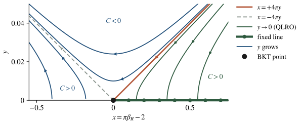
Figure 1. The Kosterlitz flow, with $C=x^2-16{\pi }^2{y}^2$. Right of the separatrix $x=+4\pi y$ ($C>0$, $x>0$): $y\to 0$, a line of Gaussian fixed points (the QLRO phase, one point per temperature). Left of it, in the wedge $C<0$ and in the region $C>0$, $x<0$: $y$ grows (vortices proliferate) and the flow exits toward the disordered phase. The trajectories are computed by integrating the linearized flow of §2.3, $dx/d\ell =-16{\pi }^2{y}^2$, $dy/d\ell =-xy$.

Three consequences, each a genuine prediction:

(i) A critical phase. For $C>0$, $x>0$ (low $T$, small $y$), the flow terminates on the fixed line $y=0$ at some $x_{\infty }=\sqrt{C}>0$: the long-distance theory is a pure Gaussian with renormalized stiffness ${\beta }_R(\infty )=(2+x_{\infty })/\pi$. Every temperature below $T_{BKT}$ is critical, with continuously varying exponent $\eta =1/2\pi {\beta }_R(\infty )$ — Week 1’s QLRO, now with the vortex renormalization included.

(ii) The universal jump [Computed]. As $T\to T_{BKT}^{-}$ along the line of initial conditions, the terminus $x_{\infty }\to 0^{+}$: the renormalized stiffness approaches

$$\underset{T\to T_{BKT}^{-}}{\lim }{\beta }_R(\infty ;T)=\frac{2}{\pi },\text{i.e.}\boxed{\frac{{\rho }_s(T_{BKT}^{-})}{k_B{T}_{BKT}}=\frac{2}{\pi },}$$

identifying ${\beta }_R={\rho }_s/k_{B}T$ with the measurable superfluid stiffness (the helicity modulus of Week 1 Problem 6, Week 3 Problem 4 and Problem 2 below). Above the transition ${\rho }_s=0$ (no QLRO): the stiffness jumps by the universal amount $2/\pi$, whatever the material, lattice, or microscopic coupling. Nelson–Kosterlitz predicted it; Bishop–Reppy’s torsional-oscillator experiment on helium films measured it. A transition with no order parameter, certified by a universal number.

(iii) The essential singularity [Computed]. Just above $T_{BKT}$, the initial condition sits slightly on the running side: $C=-bt$ with $t=(T-T_{BKT})/T_{BKT}$ small, $b>0$. Integrate the flow along such a trajectory: with $16{\pi }^2{y}^2=x^2+bt$,

$$\frac{dx}{d\ell }=-(x^2+bt)⟹\ell (x)=\frac{1}{\sqrt{bt}}[\arctan \frac{x_0}{\sqrt{bt}}-\arctan \frac{x}{\sqrt{bt}}],$$

and the total flow time before $x$ runs to $O(-1)$ (vortices dense; stop the flow) is ${\ell }^{\ast }\simeq \pi /\sqrt{bt}$. The correlation length is the scale reached:

$$\boxed{\xi \sim a_0{e}^{{\ell }^{\ast }}=a_0\exp \left(\frac{\mathrm{const}}{\sqrt{T-T_{BKT}}}\right).}$$

No power law: all thermodynamic exponents are washed out (the singular free energy $\sim {\xi }^{-2}$ has an essential singularity; specific heat is smooth through $T_{BKT}$, with only a non-singular bump above it). If a simulation or experiment fits a power-law divergence at a putative XY transition, it is measuring crossover, not asymptotics — a practical warning that follows directly from the flow.

Physical picture. The dielectric metaphor is exact enough to compute with. Below $T_{BKT}$ the vortex gas is a polarizable medium of bound pairs: it screens (reduces ${\beta }_R$) but never conducts — test charges at infinity still feel a logarithm, merely with a renormalized coefficient. At $T_{BKT}$ the largest pairs ionize, the medium becomes a plasma, screening becomes complete (Debye), and the logarithm is cut off at $\xi$: free vortices at density ${\xi }^{-2}$ destroy the stiffness entirely. The jump is the statement that a logarithmic dielectric cannot fade away continuously: either the log survives (with coefficient $\ge 2/\pi$, else pairs ionize) or it is screened to zero. Nothing in between is self-consistent — that is the physics content of the separatrix.

3. Kramers–Wannier duality of the 2d Ising model

The second duality of Block A: the Ising model equals itself at a dual temperature. Everything is a ${\mathbb{Z}}_2$ shadow of Week 3 — with the coefficient group $\mathbb{Z}$ replaced by ${\mathbb{Z}}_2$, Poisson resummation becomes the two-term Fourier transform on ${\mathbb{Z}}_2$, and the “integer currents” become the loops below.

3.1 The high-temperature expansion [Computed.]

$Z={\sum }_{\{s_x=\pm 1\}}{\prod }_{⟨xy⟩}{e}^{\beta s_x{s}_y}$ on the $L\times L$ torus: $N=L^2$ sites, $N_b=2N$ bonds, $N_p=N$ plaquettes. Use the ${\mathbb{Z}}_2$ character identity per bond:

$$e^{\beta s{s}^{\prime }}=\cosh \beta (1+ts{s}^{\prime }),t\equiv \tanh \beta .$$

Expand the product over bonds: each term selects a subset $\gamma$ of “occupied” bonds, contributing $t^{|\gamma |}{\prod }_x{s}_x^{{\mathrm{deg}}_{\gamma }(x)}$. Summing each $s_x=\pm 1$ kills every term where some site has odd degree and yields $2$ per site otherwise. The surviving subsets — every vertex of even degree — are exactly the ${\mathbb{Z}}_2$ 1-cycles of the lattice ($\partial \gamma =0$ mod 2, Week 2 language):

$$\boxed{Z=2^N(\cosh \beta {)}^{2N}\sum _{\gamma \in \ker {\partial }_1\otimes {\mathbb{Z}}_2}{t}^{|\gamma |}.}$$

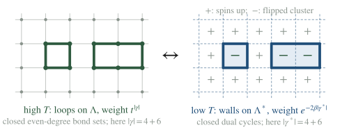
Figure 2. The two expansions that Kramers–Wannier equates: high-temperature loops on the direct lattice ↔ low-temperature domain walls on the dual lattice.

3.2 The low-temperature expansion [Computed.]

Expand instead around the two ground states. A configuration is specified by its ground state and the set of flipped-cluster boundaries: domain walls, which are even-degree bond sets on the dual lattice — ${\mathbb{Z}}_2$ 1-cycles ${\gamma }^{\ast }$ on ${\Lambda }^{\ast }$. Each wall bond costs $e^{-2\beta }$ relative to alignment:

$$Z=2e^{2N\beta }\sum _{{\gamma }^{\ast }}{e}^{-2\beta |{\gamma }^{\ast }|}\left({\gamma }^{\ast }\text{ ranging over the realizable wall classes — see §3.4}\right).$$

3.3 The duality and the self-dual point [Computed.]

Both expansions sum ${\mathbb{Z}}_2$ 1-cycles weighted by (small parameter)${}^{\mathrm{length}}$, one on Λ and one on ${\Lambda }^{\ast }$ (Figure 2), and the square lattice is self-dual. Identify the weights:

$$t=\tanh \beta ⟷e^{-2{\beta }^{\ast }}.$$

This relation is symmetric in disguise. Compute: ${\cosh }^2\beta (1-t^2)=1$ gives ${\cosh }^2\beta =1/(1-t^2)$, so

$$\sinh 2\beta =2t{\cosh }^2\beta =\frac{2t}{1-t^2},\sinh 2{\beta }^{\ast }=\frac{e^{2{\beta }^{\ast }}-e^{-2{\beta }^{\ast }}}{2}=\frac{t^{-1}-t}{2}=\frac{1-t^2}{2t},$$ $$\boxed{\sinh 2\beta \cdot \sinh 2{\beta }^{\ast }=1.}$$

High temperature at β maps to low temperature at ${\beta }^{\ast }$ and vice versa. If the model has a single phase transition (it does — Peierls plus Onsager), it must sit at the self-dual point:

$$\sinh 2{\beta }_c=1⟹{\beta }_c=\frac{1}{2}\ln (1+\sqrt{2})=0.4407\dots$$

Kramers and Wannier located $T_c$ three years before Onsager solved the model — the historical proof that duality is a computational weapon, not a curiosity.

Physical picture. What has actually been proven is a functional equation for the free energy: $F(\beta )=F({\beta }^{\ast })+\text{analytic}$. Such an equation cannot by itself create a transition; it can only constrain where one sits — a single non-analyticity must live at the equation’s fixed point. This is duality’s general epistemic status, worth internalizing now: dualities relocate and constrain singularities, while independent physics (here Peierls’ argument that a transition exists at all) supplies them. The same division of labor recurs for Wegner’s self-dual 4d gauge theory (Week 5) and for every self-dual point of Semester II.

3.4 Boundary conditions, tracked honestly [Model proof.]

The torus hides a refinement that textbooks skip and Semester II needs. The two expansions do not sum the same homology classes:

• The loop expansion (§3.1) includes cycles of every class in $H_1(T^2,{\mathbb{Z}}_2)={\mathbb{Z}}_2^2$ — nothing restricts windings.
• The wall expansion (§3.2) realizes only null-homologous walls: a wall is the boundary of the flipped region, and boundaries are trivial in homology (a band wrapped around the torus has two winding walls — total class zero mod 2). Winding-odd wall classes are unreachable by any spin configuration with periodic boundary conditions.

The fix: track the four boundary-condition sectors. Let $ϵ=({ϵ}_1,{ϵ}_2)\in {\mathbb{Z}}_2^2$ label periodic (${ϵ}_i=0$) or antiperiodic (${ϵ}_i=1$) conditions in direction $i$, where antiperiodic means a seam: the couplings of the $i$-bonds crossing one closed dual cycle, which winds in the other direction, are flipped. We write $Z_{ϵ}(\beta )$ for the partition function in sector ε; everything below holds on any $L_1\times L_2$ torus, with $N=L_1{L}_2$ sites, $2N$ bonds and $N$ plaquettes. A loop γ of class $[\gamma ]=({\gamma }_1,{\gamma }_2)\in H_1(T^2,{\mathbb{Z}}_2)$ crosses the seams ${ϵ}_1{\gamma }_1+{ϵ}_2{\gamma }_2$ times mod 2, so in the loop expansion each loop carries the sign of the evaluation of the sector label, a class in $H^1(T^2,{\mathbb{Z}}_2)$, on its homology class:

$$Z_{ϵ}(\beta )=2^N(\cosh \beta {)}^{2N}\sum _{\gamma }{t}^{|\gamma |}(-1{)}^{ϵ\cdot [\gamma ]},ϵ\cdot [\gamma ]\equiv {ϵ}_1{\gamma }_1+{ϵ}_2{\gamma }_2(\mathrm{mod}2).$$

In the wall expansion the seam changes which wall class is realizable. Follow the spins once around a closed loop $C$ of their own lattice: they return to their starting values, so $C$ crosses the walls an odd number of times exactly when it contains an odd number of flipped couplings, that is, when $\widetilde{ϵ}\cdot [C]=1$ in the sector $\widetilde{ϵ}$. The walls of that sector therefore form a cycle whose intersection number with every class $c$ is ${\widetilde{ϵ}}_1{c}_1+{\widetilde{ϵ}}_2{c}_2$, and since the intersection form of Week 2 §8 pairs $(w_1,w_2)$ with $(c_1,c_2)$ as $w_1{c}_2+w_2{c}_1$, the wall class is $({\widetilde{ϵ}}_2,{\widetilde{ϵ}}_1)$: antiperiodicity in direction 1 forces a wall that winds along direction 2, and vice versa. The leading entries of the bookkeeping, on an $L\times L$ torus (classes labelled by winding $[\gamma ]\in {\mathbb{Z}}_2^2$; shortest representative lengths shown):

contribution	class	length	weight in $Z_{ϵ}$ (loop expansion)
empty configuration	$(0,0)$	0	$+1$, every sector
smallest plaquette loop	$(0,0)$	4	$+t^4$, every sector
straight $x$-winding loop	$(1,0)$	$L$	$(-1{)}^{{ϵ}_1}{t}^L$
straight $y$-winding loop	$(0,1)$	$L$	$(-1{)}^{{ϵ}_2}{t}^L$
both windings (crossed)	$(1,1)$	$2L$	$(-1{)}^{{ϵ}_1+{ϵ}_2}{t}^{2L}$

Trivial-class terms enter every sector with the same sign; winding terms flip sign across sectors, so sector sums project onto homology classes: ${\sum }_{ϵ}(-1{)}^{ϵ\cdot h}{Z}_{ϵ}$ keeps exactly the class-$h$ loops. Matching the two representations sector by sector gives the duality as a ${\mathbb{Z}}_2$ Fourier transform on $H_1$, prefactor included. With $P_h(t)\equiv {\sum }_{[\gamma ]=h}{t}^{|\gamma |}$ the loop sum of class $h$, the loop expansion inverts, through ${\sum }_{ϵ}(-1{)}^{ϵ\cdot (h+h^{\prime })}=4{\delta }_{h,h^{\prime }}$, to

$$P_h(t)=\frac{1}{4\cdot 2^N{\cosh }^{2N}\beta }\sum _{ϵ\in {\mathbb{Z}}_2^2}(-1{)}^{ϵ\cdot h}{Z}_{ϵ}(\beta ),$$

while the wall expansion of the dual model, an Ising model on ${\Lambda }^{\ast }$ at coupling ${\beta }^{\ast }$ (again an $L_1\times L_2$ torus, with $N$ sites and $2N$ bonds), is in the sector $\widetilde{ϵ}$ a sum over walls on Λ of the single class $({\widetilde{ϵ}}_2,{\widetilde{ϵ}}_1)$, with two spin configurations per wall configuration:

$${\tilde{Z}}_{\widetilde{ϵ}}({\beta }^{\ast })=2e^{2N{\beta }^{\ast }}{P}_{({\widetilde{ϵ}}_2,{\widetilde{ϵ}}_1)}\left(e^{-2{\beta }^{\ast }}\right).$$

With $e^{-2{\beta }^{\ast }}=t$ we have $e^{2N{\beta }^{\ast }}={\coth }^N\beta$ and $2{\coth }^N\beta /(4\cdot 2^N{\cosh }^{2N}\beta )=1/[2(2\sinh \beta \cosh \beta {)}^N]$, so that

$$\boxed{{\tilde{Z}}_{\widetilde{ϵ}}({\beta }^{\ast })=\frac{1}{2{\sinh }^{N}2\beta }\sum _{ϵ\in {\mathbb{Z}}_2^2}(-1{)}^{{ϵ}_1{\widetilde{ϵ}}_2+{ϵ}_2{\widetilde{ϵ}}_1}{Z}_{ϵ}(\beta ),}$$

exactly, on every $L_1\times L_2$ torus with $L_1,L_2\ge 2$. The sign is the evaluation of ε on the realizable wall class, $ϵ\cdot ({\widetilde{ϵ}}_2,{\widetilde{ϵ}}_1)$, which is the mod-2 intersection form of the two sector labels. Note that the placement of the indices matters: the dot pairing $(-1{)}^{ϵ\cdot \widetilde{ϵ}}$ gives the same numbers on the square torus only because a rotation by 90° exchanges the two directions there, and it fails as soon as $L_1\ne L_2$. We checked the boxed identity by exhaustive enumeration of all four sectors on both sides of the $2\times 3$, $3\times 3$, $3\times 4$ and $2\times 5$ tori, where it holds to machine precision while the dot pairing fails on every non-square one. For instance, the shortest $x$-winding loop (class $(1,0)$, length $L_1$) survives only in the dual sector with $({\widetilde{ϵ}}_2,{\widetilde{ϵ}}_1)=(1,0)$, that is, $\widetilde{ϵ}=(0,1)$, whose antiperiodicity in direction 2 forces a wall along direction 1: the wall-realizability rule, sector by sector. $\square$

Two lessons: (i) dualities act on the space of boundary conditions/sectors, generally mixing them by a discrete Fourier transform on homology — in Semester II this becomes “gauging maps the theory to its orbifold, and the sectors are the background holonomies”; (ii) the pairing between the direct and the dual sector labels is once again the intersection form, the same “+1” of Week 2, Figure 3, while the sign a single loop picks up in a given sector is the evaluation $(-1{)}^{ϵ\cdot [\gamma ]}$. The two are related by Poincaré duality, which turns the label ε into the class $({ϵ}_2,{ϵ}_1)$ of its seam, so that $ϵ\cdot [\gamma ]$ is the intersection number of γ with the seam.

4. Kadanoff–Ceva disorder operators

Duality exchanges the spin ${\sigma }_x$ with an object living on dual sites: the disorder operator ${\mu }_{\tilde{x}}$.

4.1 Definition and well-definedness [Computed.]

${\mu }_{\tilde{x}}{\mu }_{\tilde{y}}$ is defined by flipping the coupling $\beta \to -\beta$ on every bond crossed by a chosen dual path (“seam”) $\tilde{\gamma }$ from $\tilde{x}$ to $\tilde{y}$, as in Figure 3:

$$⟨{\mu }_{\tilde{x}}{\mu }_{\tilde{y}}⟩=\frac{Z[\beta \to -\beta \text{ on }\tilde{\gamma }]}{Z}.$$

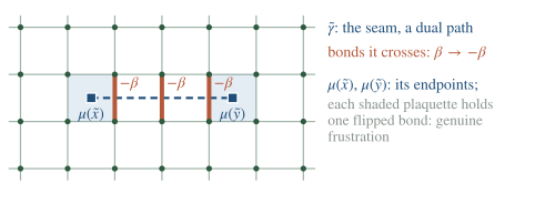
Figure 3. A disorder-operator pair: a seam of flipped bonds ($\beta \to -\beta$) joining two dual sites; only the two endpoint plaquettes are frustrated.

The seam is unobservable; its endpoints are not. Deform $\tilde{\gamma }$ to ${\tilde{\gamma }}^{\prime }$ across a site $x$: the two seams differ by the set of bonds around $x$, and flipping all couplings at one site is undone by the change of variables $s_x\to -s_x$ — a ${\mathbb{Z}}_2$ “gauge transformation” of the dummy spins. Thus $⟨\mu \mu ⟩$ depends only on $\tilde{x},\tilde{y}$ [Computed]. What cannot be gauged away are the endpoints: there the frustration is genuine (an odd plaquette of flipped bonds), and that is where the physics sits. This seam/endpoint dichotomy is the prototype for every extended operator in the course — Dirac strings (Week 8), ‘t Hooft lines (Week 11), symmetry defects (Semester II).

4.2 The disorder correlator is the dual order correlator [Computed.]

Re-run the duality of §3 with the seam inserted; the weight bookkeeping is worth displaying. In the wall expansion of $Z[\beta \to -\beta \text{ on }\tilde{\gamma }]$, examine one seam bond: if no wall crosses it, the two spins agree and the flipped coupling costs $e^{-\beta }/e^{+\beta }=e^{-2\beta }$ relative to normal; if a wall does cross, the spins disagree and the flipped coupling gains $e^{+2\beta }$ relative to what a wall bond normally pays. Summarizing, with $u\equiv e^{-2\beta }$:

bond type	no wall	wall
normal	$1$	$u$
seam	$u$	$1$

The seam rewards walls: relabeling the wall variable on each seam bond (wall ↔ no-wall) restores the normal weights everywhere at the cost of changing the wall parity constraint precisely at the seam’s endpoints — the sum becomes one over wall configurations with a single open wall ending at $\tilde{x}$ and $\tilde{y}$. But “open high-temperature graphs from $\tilde{x}$ to $\tilde{y}$ with weight $u^{|\gamma |}$” is exactly the §3.1 expansion of the spin–spin correlator on the dual lattice at the coupling ${\beta }^{\ast }$ with $\tanh {\beta }^{\ast }=u=e^{-2\beta }$ — the KW relation again. Therefore, exactly:

$$\boxed{⟨{\mu }_{\tilde{x}}{\mu }_{\tilde{y}}{⟩}_{\beta }=⟨{\sigma }_{\tilde{x}}{\sigma }_{\tilde{y}}{⟩}_{{\beta }^{\ast }}.}$$

Consequences, read from known Ising behavior:

$$T<T_c:⟨\mu \mu ⟩\stackrel{|\tilde{x}-\tilde{y}|\to \infty }{\to }0(\text{disorder "uncondensed"}),T>T_c:⟨\mu \mu ⟩\to m^{\ast }({\beta }^{\ast }{)}^2\ne 0(\text{disorder condensed}),$$

the exact mirror of $⟨\sigma \sigma ⟩$. The high-temperature phase, featureless to every local operator, has long-range order of a non-local operator. Phases invisible to Landau are visible to disorder operators — the diagnostic pattern of the entire course (Wegner’s phases next week are distinguished exactly this way).

The complete dictionary of “what condenses where,” assembled for later reuse:

	$⟨\sigma \sigma ⟩$	$⟨\mu \mu ⟩$	fermion $\psi =\sigma \mu$	phase name
$T<T_c$	$\to m^2\ne 0$	$\to 0$	massive	ordered (“μ confined”)
$T=T_c$	$r^{-1/4}$	$r^{-1/4}$	massless	self-dual critical point
$T>T_c$	$\to 0$	$\to {\tilde{m}}^2\ne 0$	massive	disordered (“σ confined”)

Order and disorder cannot condense simultaneously — their mutual semi-locality (§4.3) forbids it (a nonzero $⟨\sigma ⟩$ and $⟨\mu ⟩$ would contradict the crossing sign at long distance). Exactly one of the pair condenses in each gapped phase, and the critical point is where custody changes. This exclusivity — mutually non-local operators cannot both condense — recurs as the Wilson/‘t Hooft perimeter-law dichotomy of gauge theory (Week 5 onward) and as the anyon-condensation logic of Semester II. The Ising model is its two-state prototype.

4.3 The order–disorder algebra, and a fermion [Computed.]

Sharpest in the transfer-matrix (quantum spin chain) language, where the 2d classical model becomes the transverse-field Ising chain with Hilbert space ${⨂}_i{\mathbb{C}}^2$ and

$${\sigma }_i={\sigma }_i^z,{\mu }_{\tilde{ı}}=\prod _{j\le i}{\sigma }_j^x$$

(the disorder operator = flip all spins to the left of the dual site $\tilde{ı}$ — the operator version of the seam). Two Pauli computations:

Mutual semi-locality. For any site $k$ and dual site $\tilde{ı}$:

$${\sigma }_k^z{\mu }_{\tilde{ı}}=\left(\prod _{j\le i}{\sigma }_j^x\right){\sigma }_k^z\times \{\begin{array}{ll}(-1)& k\le i(\text{the seam crosses }k)\\ (+1)& k>i\end{array}$$

directly from ${\sigma }^z{\sigma }^x=-{\sigma }^x{\sigma }^z$ at the crossing site. Order and disorder operators are mutually non-local: each is charged under the symmetry the other generates (μ is a half-space ${\mathbb{Z}}_2$ transformation; σ is ${\mathbb{Z}}_2$-odd). Neither is “more fundamental.”

The composite is a fermion. Pair the order operator at site $i$ with the disorder operator at the dual site to its left:

$${\psi }_i={\mu }_{i-\frac{1}{2}}{\sigma }_i^z=\left(\prod _{j<i}{\sigma }_j^x\right){\sigma }_i^z,{\bar{\psi }}_i=\left(\prod _{j<i}{\sigma }_j^x\right){\sigma }_i^y$$

(string strictly to the left — pairing with ${\mu }_{i+\frac{1}{2}}$ instead would put a ${\sigma }_i^x$ on top of the ${\sigma }_i^z$ and spoil Hermiticity by a stray factor of $i$). These are Hermitian and square to one: Majorana operators. Anticommutation, for $i<k$:

$${\psi }_i{\psi }_k=-{\psi }_k{\psi }_i,$$

because exactly one crossing occurs — ${\psi }_k$‘s string ${\prod }_{j<k}{\sigma }_j^x$ contains ${\sigma }_i^x$, which anticommutes with ${\psi }_i$‘s ${\sigma }_i^z$, while ${\psi }_i$‘s string ends before site $k$ [Computed]. These are the Jordan–Wigner Majorana fermions, and the “string” that makes a fermion out of two bosonic operators is the disorder seam.

Physical picture. Statistics is not an intrinsic property of a particle here — it is a relational property of operator pairs. σ alone is bosonic; μ alone is bosonic; their bound state is a fermion because each factor is charged under the symmetry whose defect the other creates, and exchanging two composites forces one seam-crossing sign. This “statistics from mutual linking” is the exact mechanism by which the toric code’s $e$–$m$ bound state $\epsilon$ is a fermion (Semester II Week 8), and — in its continuum dress — by which flux–charge composites anywhere acquire anyonic phases. The Ising chain is the smallest laboratory where one can compute it, which is why we did. The free-fermion solvability of the 2d Ising model (Onsager, in modern dress) is the statement that $\psi$ has a quadratic Hamiltonian. We will not solve it here; the point for this course is structural: order × disorder = fermion is the first instance of the anyon/statistics-from-mutual-linking phenomenon that Semester II Week 8 develops for the toric code.

4.4 Duality as an operator: the defect preview [Computed, with the normalization and one sign fixed numerically; the explicit construction is Semester II Week 13.]

In chain language, Kramers–Wannier is the map of bond algebras

$${\sigma }_i^x⟼{\sigma }_i^z{\sigma }_{i+1}^z,{\sigma }_i^z{\sigma }_{i+1}^z⟼{\sigma }_{i+1}^x,$$

which exchanges the transverse-field Ising Hamiltonian $H(g)=-\sum ({\sigma }^z{\sigma }^z+g{\sigma }^x)$ with $H(1/g)$ (up to rescaling) — fixed point at $g=1$, the chain avatar of $\sinh 2{\beta }_c=1$. One can ask for the operator $D$ implementing the map, defined on the periodic chain of $N$ sites by

$$D{\sigma }_i^x={\sigma }_i^z{\sigma }_{i+1}^{z}D,D{\sigma }_i^z{\sigma }_{i+1}^z={\sigma }_{i+1}^{x}D(i+N\equiv i),$$

so that $DH(g)=gH(1/g)D$. These relations fix $D$ up to a scale, and $D$ cannot be unitary; counting states shows why. Deep in the ordered phase ($g\ll 1$) the low-energy states are the symmetric and antisymmetric combinations $|\uparrow \cdots \uparrow ⟩\pm |\downarrow \cdots \downarrow ⟩$, two nearly degenerate states with ${\mathbb{Z}}_2$ charges $\eta =\pm 1$, the eigenvalues of $\eta ={\prod }_i{\sigma }_i^x$. The dual Hamiltonian $gH(1/g)$ is then deep in its paramagnetic phase and has a single ground state. The map matches the ${\mathbb{Z}}_2$-even spectra of $H(g)$ and $gH(1/g)$ level by level, but it has nothing in the periodic chain to match the odd states onto: their partners are the even states of the chain with an antiperiodic boundary bond, the sector mixing of §3.4 in chain language. Precisely, $D$ is injective on the ${\mathbb{Z}}_2$-even sector, which it maps onto itself, and annihilates the odd sector, $D\eta =\eta D=D$ (Problem 6⋆). The resolution is that $D$ is non-invertible, obeying the fusion rule

$$D\times \bar{D}=1+\eta ,\eta =\prod _i{\sigma }_i^x$$

(the fusion algebra of the defect lines: unnormalized sum of the identity line and the symmetry line). The Hilbert-space counterpart is

$$D^{†}D=1+\eta =2P_{\mathrm{even}},P_{\mathrm{even}}=\frac{1}{2}(1+\eta ),$$

proportional to — not equal to — the projector onto the ${\mathbb{Z}}_2$-even sector: $D$ annihilates the odd sector outright. (Keep the two statements distinct: fusion rules of topological lines carry no normalization; operator identities do. Conflating them produces “projectors” that fail to square to themselves.) On the lattice the square of $D$ carries a translation. Squaring the defining relations gives $D^2{\sigma }_i^x={\sigma }_{i+1}^x{D}^2$ and $D^2{\sigma }_i^z{\sigma }_{i+1}^z={\sigma }_{i+1}^z{\sigma }_{i+2}^z{D}^2$, so $T^{-1}{D}^2$ commutes with every bond operator, where $T$ is the translation by one site, $T{\sigma }_i{T}^{-1}={\sigma }_{i+1}$. The bond operators generate all ${\mathbb{Z}}_2$-even operators, whose commutant is spanned by $1$ and η, so that $T^{-1}{D}^2=c_1+c_2\eta$; $D\eta =D$ gives $c_1=c_2$, and $(D^2{)}^{†}{D}^2=D^{†}(1+\eta )D=2(1+\eta )$, which uses $\eta D=D$, gives $|c_1|=1$. With the phase of $D$ chosen so that its matrix is real in the ${\sigma }^z$ basis,

$$D^2=(1+\eta )T,$$

where $T$ appears because each application of the map moves the bond variables half a site to the right. Since $D$ also commutes with $T$ (translation covariance of the defining relations gives $T^{-1}DT=\pm D$, and the numerical solution of the next sentence gives the plus sign), comparison with $D^{†}D=1+\eta$ gives $D^{†}=T^{-1}D$: on the lattice the conjugate line $\bar{D}$ is $D$ followed by a translation. We solved the defining relations numerically for $N=3,\dots ,6$ and confirmed every statement of this paragraph and of the two preceding ones, including the level-by-level matching of the even spectra and the antiperiodic partners of the odd ones. Geometrically, $D$ is a topological defect line in the 2d model (Aasen–Mong–Fendley), and “the model is self-dual” becomes “the model contains a topological line with projector fusion.” Constructing $D$ explicitly and computing this fusion is Semester II Week 13’s mini-calculation; here it stands as Block A’s closing thought: every duality we have performed is secretly an operator inside the theory it acts on.

5. Subtleties and fine print

F1 — The jump, operationally. For a helium film, ${\beta }_R={\hslash }^2{\rho }_s/(m^2{k}_{B}T)$ in laboratory units, and the prediction reads ${\rho }_s(T_{BKT}^{-})/T_{BKT}=\frac{2}{\pi }\frac{m^2{k}_B}{{\hslash }^2}$ — a combination of fundamental constants, independent of the substrate and film thickness. Bishop–Reppy’s torsional oscillator confirmed both the value and its universality across films. Few statistical-mechanics predictions this sharp exist; it is the experimental signature that BKT physics is real and not a lattice artifact.

F2 — Is the dilute-gas RG self-consistent for the XY model? The flow was derived to $O(y^2)$; it is trustworthy only if $y$ is small near the transition. Estimate it from Week 3’s long-distance matching (that fugacity is a normalization convention at the lattice scale, not an exact microscopic quantity — Week 3, Move 7): evaluating at the marginality stiffness $\pi {\beta }_R=2$, $y\sim e^{-2{\pi }^2{\beta }_R\kappa }=e^{-4\pi \kappa }\approx e^{-3.2}\approx 0.04$ — small enough that the dilute expansion is self-consistent for the Villain model, with short-distance corrections shifting the number at the tens-of-percent level, not its smallness. Models with genuinely low vortex core costs (e.g. modified XY actions) can push $y$ large and convert the transition to first order [Stated — refs: Minnhagen, Rev. Mod. Phys. 59 (1987) 1001]; the sine-Gordon universality holds only in the dilute basin.

F3 — What "${\beta }_R$" is measured by. The flow variable ${\beta }_R(\infty )$ is the coefficient of the long-distance logarithm — operationally the helicity modulus/stiffness (twisted boundary conditions: Week 3 Problem 4, and Problem 2 below, where the twist enters the tilt sectors as a phase), not the bare coupling and not directly the exponent of any single microscopic correlator. Comparing simulations to the RG means comparing stiffnesses. (The correlator exponent is then $\eta =1/2\pi {\beta }_R$.)

F4 — Kramers–Wannier needs the square lattice’s self-duality. On the triangular lattice, duality maps to the honeycomb and back; locating $T_c$ then requires the star–triangle relation in addition. Self-duality is a happy accident of the square lattice; duality itself (the loop/wall Fourier transform of §3.4) is completely general — and it is the general statement that survives into Semester II.

F5 — ⟨μ⟩ alone requires care. A single disorder operator needs a seam to the boundary (or a partner); on the torus only pairs (or an even number) are defined — the ${\mathbb{Z}}_2$ version of “charge neutrality on compact space” from Week 3, F4. Statements like ”$⟨\mu ⟩\ne 0$ in the disordered phase” implicitly mean the cluster-decomposed limit ${\lim }_{|\tilde{x}-\tilde{y}|\to \infty }\sqrt{⟨\mu \mu ⟩}$.

F6 — The homology bookkeeping is physics, not pedantry. The sector Fourier transform of §3.4 is exactly the structure that reappears as: modular covariance of sector partition functions; discrete gauging = summing sectors (Semester II Week 4); and the fermion’s need for spin structures (the JW string of §4.3 is sector-sensitive — Problem 5). Skipping it produces wrong factors of 2 in every one of those places.

6. Common misconceptions

• “BKT spontaneously breaks the U(1) symmetry.” Nothing breaks: $⟨\vec{S}⟩=0$ on both sides (Mermin–Wagner, Week 1). The transition separates two symmetric phases distinguished by stiffness and defect binding — the founding example of order beyond Landau.
• “Below $T_{BKT}$ there are no vortices.” Bound pairs exist at every $T>0$ with computable density $\sim y^2$; they are why ${\beta }_R<\beta$. What vanishes below the transition is the density of free vortices.
• ”$\xi$ diverges with some exponent ν.” No power law exists: $\xi \sim e^{c/\sqrt{t}}$ (§2.3). Finite-size or crossover fits produce effective “exponents” that drift with the fitting window — a well-documented trap in the simulation literature.
• “The disorder operator is unphysical because it depends on an arbitrary seam.” Its correlators are seam-independent (§4.1) — exactly as gauge-dependent intermediate quantities produce gauge-invariant observables. The seam teaches, rather: extended unobservable strings with observable endpoints are how mutually non-local operator pairs coexist in one theory.

7. Historical note

Berezinskii (1971) and Kosterlitz–Thouless (1973) independently identified defect unbinding as a phase transition compatible with Mermin–Wagner; Kosterlitz (1974) supplied the RG, and Nelson–Kosterlitz (1977) extracted the universal jump, confirmed by Bishop–Reppy (1978). On the other strand: Kramers–Wannier (1941) found the duality and $T_c$; Onsager (1944) solved the model; Kadanoff–Ceva (1971) introduced disorder variables and the order–disorder algebra, explicitly anticipating the operator content of lattice gauge theories — Wegner’s paper (Week 5) appeared the same year, and Fradkin–Susskind (1978) unified the two strands in the Hamiltonian language used in §4.3. The 2016 Nobel Prize (Thouless, Haldane, Kosterlitz) recognized, in large part, the circle of ideas in §§1–2.

8. What to take away

1. The BKT flow is two equations with hyperbolic trajectories: $dy/d\ell =(2-\pi {\beta }_R)y$ [derived from the Week-3 operator dimension] and $d{\beta }_R^{-1}/d\ell =4{\pi }^3{y}^2$ [screening, derived with its constant, to $O(y^2)$]. The trajectories terminate on a fixed line (QLRO) or run away (plasma).
2. Two universal signatures, both derived from the flow: the stiffness jump ${\rho }_s/T_{BKT}=2/\pi$ and the essential singularity $\xi \sim e^{c/\sqrt{T-T_{BKT}}}$; both measured, neither Landau-describable.
3. Kramers–Wannier is the ${\mathbb{Z}}_2$ Fourier transform of Week 3’s duality: loops ↔ walls, $\sinh 2\beta \sinh 2{\beta }^{\ast }=1$, $T_c$ located without solving the model — and on the torus the duality acts on boundary-condition sectors through the intersection form.
4. Disorder operators complete the operator content: $⟨\mu \mu {⟩}_{\beta }=⟨\sigma \sigma {⟩}_{{\beta }^{\ast }}$ [derived], order and disorder are mutually semi-local, their composite is the Jordan–Wigner fermion, and the duality itself is a non-invertible defect line — the seed sentence of Semester II.

9. Looking ahead: Block B

Week 5 gauges. Wegner’s construction promotes the Ising ${\mathbb{Z}}_2$ to a local symmetry, Elitzur’s theorem wipes out every local order parameter, and the model’s two phases — provably distinct — are distinguishable only by the behavior of a loop: Wilson’s criterion, four years before Wilson used it for quarks. The disorder operator of this week becomes the ‘t Hooft loop; the Fourier-on-sectors structure becomes the electric/magnetic flux sectors of gauge theory. Block A built the tools on spin systems; Block B aims them at gauge fields, where they were always headed.

10. Problem set

Problems 1–4 are the classroom core and are solvable from this note and the Week 3 results it quotes; 5⋆ and 6⋆ are self-study consolidation, each with its method indicated; 7⋆⋆ and 8⋆⋆ are research extensions, each stating what is known, what is explored, its sources and what counts as completion.

Core problems (everyone).

1. Flow-diagram quantitative work. (a) §2.3 integrates the flow explicitly only above $T_{BKT}$. Consider instead a trajectory below it, with $C=x_{\infty }^2>0$ and $x_0>0$, and use the conservation of $C$ to show that

$$x(\ell )=x_{\infty }\coth [x_{\infty }(\ell +{\ell }_0)],4\pi y(\ell )=\frac{x_{\infty }}{\sinh [x_{\infty }(\ell +{\ell }_0)]},\coth (x_{\infty }{\ell }_0)=\frac{x_0}{x_{\infty }},$$

so that at large scales $y\propto (r/a{)}^{-x_{\infty }}$ and ${\beta }_R(r)-{\beta }_R(\infty )\propto (r/a{)}^{-2x_{\infty }}$. Identify $-x_{\infty }$ with the RG eigenvalue $2-\pi {\beta }_R(\infty )$ of the vortex fugacity on the fixed line, and check that the limit $x_{\infty }\to 0$ reproduces the critical trajectory of (c). (b) A sample has bare couplings such that $x_0=0.1$, $y_0=0.005$ at scale $a_0$. Which phase is it in? Compute its ${\beta }_R(\infty )$ or its $\xi$, as appropriate. (c) Show that on the critical trajectory $y(\ell )=y_0/(1+4\pi y_0\ell )$ — logarithmically slow decay — and deduce the multiplicative logarithmic correction to the spin correlator at exactly $T_{BKT}$ [famously $⟨\vec{S}\vec{S}⟩\sim r^{-1/4}(\ln r{)}^{1/8}$; derive the mechanism, quote the exponent].

2. The jump from the helicity modulus. This problem rests on the current representation of Week 3 §2 and its tilt sectors (Week 3 §3). On the $L\times L$ torus impose the twist ${\theta }_{x+L\hat{1}}={\theta }_x+\alpha$ and define the helicity modulus by ${\rm Y}={\partial }_{\alpha }^{2}F(\alpha ){|}_{\alpha =0}$, with $F(\alpha )=-\ln Z(\alpha )$ (Week 1 Problem 6). (a) Move the twist onto a seam, $(d\theta {)}_{\ell }\to (d\theta {)}_{\ell }+\alpha$ on the $x$-links that cross one closed dual cycle winding in the $y$-direction, and repeat the Hubbard–Stratonovich step of Week 3 §2. Show that the twist enters as the phase $e^{i\alpha w_1}$ on each current configuration, with $w_1$ the net current through the seam (the tilt $w_1$ of Week 3 §3), and conclude that ${\rm Y}=⟨w_1^2⟩$ exactly in the Villain model. (b) At the Gaussian level of Week 3 §3 the tilt weights are $e^{-w^2/2\beta }$ per direction. Poisson-resum with the identity of conventions §3,

$$\sum _{w\in \mathbb{Z}}{e}^{-w^2/2\beta +i\alpha w}=\sqrt{2\pi \beta }\sum _{k\in \mathbb{Z}}{e}^{-\beta (\alpha -2\pi k{)}^2/2},$$

and show that ${\rm Y}=\beta -4{\pi }^2{\beta }^2⟨k^2⟩$, where $⟨k^2⟩$ is the mean of $k^2$ with weights $e^{-2{\pi }^2\beta k^2}$: the spin-wave value ${\rm Y}=\beta$, up to terms of order ${\beta }^2{e}^{-2{\pi }^2\beta }$. Show also that a shift $w_1\to w_1+\alpha /2\pi$ in place of the phase would give an exponentially small Υ. (c) Take as the working hypothesis (the finite-size form of F3) that on the $L\times L$ torus the bound pairs up to size $L$ replace β by the running stiffness ${\beta }_R({\ell }_L)$, ${\ell }_L=\ln (L/a)$, in the tilt weights. Use the critical trajectory of Problem 1(c) to show that at $T_{BKT}$ the data should be compared to

$${\rm Y}(L)=\frac{2}{\pi }(1+\frac{1}{2\ln (L/L_0)}),$$

up to corrections of order $e^{-4\pi }$, where $L_0$ is fixed by the initial condition. Thus the jump of §2.3(ii) is the statement that screening lowers Υ from its Gaussian value β to ${\beta }_R$, with $\pi {\beta }_R=2$ at the transition. Explain why reading $T_{BKT}$ off the crossing ${\rm Y}(L,T)=2/\pi$ at fixed $L$, ignoring the logarithm, misidentifies it, and in which direction.

3. Kramers–Wannier with a magnetic field. Add $h{\sum }_x{s}_x$. Show the duality maps it to a seam-condensation term (a sum over disorder-line insertions) rather than a dual magnetic field, and conclude that self-duality is broken for $h\ne 0$ — consistent with the transition becoming a crossover. What operator is dual to $h\sigma$? (Answer in the language of §4: the field couples to the order operator; its dual couples to μ.)

4. Disorder correlator at criticality. At $\beta ={\beta }_c$, use $⟨\mu \mu {⟩}_{\beta }=⟨\sigma \sigma {⟩}_{{\beta }^{\ast }}$ and the known Ising exponent ${\eta }_{\mathrm{Ising}}=1/4$ to fix the decay of $⟨\mu \mu ⟩$. Both σ and μ have dimension $1/8$ at the self-dual point: what symmetry of the critical theory exchanges them, and what does that predict for the fermion ψ’s dimension? (Check: $1/8+1/8$ vs the free-fermion value $1/2$ — resolve the discrepancy by identifying which fusion channel the fermion sits in.)

Starred problems.

5⋆. Spin structures from the Jordan–Wigner string. On a periodic chain of $N$ sites, show that the fermion ${\psi }_i$ of §4.3 obeys ${\psi }_{i+N}=-\eta {\psi }_i$-type boundary conditions: the fermionic sectors (NS/R — antiperiodic/periodic) are tied to the ${\mathbb{Z}}_2$ charge sectors η. Connect to the four bosonic sectors of §3.4: this is the 2d Ising model’s spin-structure sum in microscopic form. (Hint: in the bulk ${\sigma }_i^z{\sigma }_{i+1}^z=i{\bar{\psi }}_i{\psi }_{i+1}$. Write the boundary bond ${\sigma }_N^z{\sigma }_1^z$ through ${\bar{\psi }}_N$ and ${\psi }_1$, using ${\prod }_{j<N}{\sigma }_j^x=\eta {\sigma }_N^x$, and show that it takes the bulk form with ${\psi }_{N+1}=-{\psi }_1\eta$; the order matters, and on a sector of definite η this is the stated boundary condition.)

6⋆. The defect commutes with the transfer matrix. Take the duality map of §4.4 at the self-dual point $g=1$ and verify on generators that any operator $D$ satisfying the intertwining relations commutes with $H(1)$. Then show that $D$ must annihilate the ${\mathbb{Z}}_2$-odd sector and that $D^{†}D$ is proportional to the projector onto the even one: the non-invertibility follows from pure representation theory, before any explicit construction. (Hint: multiply the intertwining relations over all $N$ sites, noting that on the periodic chain ${\prod }_i{\sigma }_i^z{\sigma }_{i+1}^z=1$; for $D^{†}D$, use the adjoint relations to show that it commutes with every bond operator, and then the commutant argument of §4.4. The ground-state count of §4.4 is a check. The construction itself: Semester II Week 13.)

⋆⋆ problems (research extension).

7⋆⋆ (optional). The ${\mathbb{Z}}_N$ clock ladder. What is known: the Villain form of the ${\mathbb{Z}}_N$ clock model is self-dual, and for $N\ge 5$ two BKT-like transitions bound an intermediate critical phase, while for $N\le 4$ there is a single transition (José, Kadanoff, Kirkpatrick and Nelson, Phys. Rev. B 16 (1977) 1217; Week 3 Problem 6⋆⋆). What is explored is this week’s sector and disorder-operator bookkeeping in ${\mathbb{Z}}_N$ form. Combine Week 3 Problem 6⋆⋆ with this week: for the ${\mathbb{Z}}_N$ clock model, derive the sector-mixing rule of §3.4 (now a ${\mathbb{Z}}_N$ Fourier transform on $H_1(T^2,{\mathbb{Z}}_N)$), identify the $N$ disorder operators, and, for $N\ge 5$, describe how the two transitions bound a critical phase in which both order and disorder correlators decay algebraically. Tabulate which operators condense in each of the three phases; this table is the $N$-state warm-up for the phase classification language of Semester II. Completion: the ${\mathbb{Z}}_N$ sector formula with its prefactor, checked by enumeration on a small torus for $N=3$; the seam weights of the disorder operators; and the three-phase table, each entry justified by the dimension counting of Week 3 Problem 6⋆⋆.

8⋆⋆ (optional). The Kosterlitz flow at next order. What is known: beyond the order of §2 the flow acquires cubic terms, and Amit, Goldschmidt and Grinstein (J. Phys. A 13 (1980) 585) found that they bring in one new universal quantity. Pelissetto and Vicari (Phys. Rev. E 87 (2013) 032105, arXiv:1212.2322, eqs. (17)–(20)) showed that analytic redefinitions of the couplings, with $v\simeq x$ and $u\simeq 4\pi y$ at leading order, bring the flow to the canonical form $du/d\ell =-uv$, $dv/d\ell =-u^2[1+b_{0}v+O(v^3)]$ with $b_0=3/2$. The jump $2/\pi$, the exponent $\frac{1}{2}$ of the essential singularity and the $(\ln r{)}^{1/8}$ of Problem 1(c) are fixed at leading order and do not change. What $b_0$ fixes are the subleading logarithms: on the critical trajectory $x(\ell )=1/(\ell +\frac{1}{2}\ln \ell +\text{const})+\dots$, which turns the result of Problem 2 into ${\rm Y}(L)={{\rm Y}}^{\ast }+C_{{\rm Y}}/(\mu +\frac{1}{2}\ln \mu )$ with $\mu =\ln (L/L_0)$, ${{\rm Y}}^{\ast }=0.636508$ and $C_{{\rm Y}}=0.318899$ on the square periodic lattice (their eq. (67), with the values of Hasenbusch 2005). What is explored: (a) without the linearization ${\beta }_R\simeq 2/\pi$ of §2.3, the flow of §2 reads $dx/d\ell =-4{\pi }^2{y}^2(2+x{)}^2$; show that it conserves $I=2{\pi }^3{y}^2-2{\beta }_R^{-1}+\pi \ln {\beta }_R^{-1}$, with $\frac{8}{\pi }(I-I{|}_{x=y=0})=-C+\frac{2}{3}{x}^3+O(x^4)$, so that its separatrix bends away from $x=4\pi y$ while keeping its endpoint and its tangent there. (b) Write the general cubic flow allowed by the fixed line and by $y\to -y$, namely $dx/d\ell =-Y^2+ax{Y}^2$ and $dY/d\ell =-xY+b{Y}^3+e{x}^{2}Y$ with $Y=4\pi y$, and show that under $x\to x+p{x}^2+q{Y}^2$, $Y\to Y(1+rx)$ the combination $a+2b+2e$ is invariant while $b$ and $e$ can be removed, so that $b_0=-(a+2b+2e)$; conclude that the curvature of the separatrix depends on the variables while its endpoint, and with it the jump, does not. (c) Integrate the canonical critical trajectory and derive the $\frac{1}{2}\ln \ell$. Sources: the two papers above and Hasenbusch (2005). Completion: (a)–(c) derived in the note’s variables; the relation $b_0=1-2b$ for the scheme of §2, where $a=-1$ and $e=0$, which fixes the $y^3$ term of $dy/d\ell$ that an independent next-order calculation in that scheme must find; and the fit of Problem 2 redone on a model flow with the $\frac{1}{2}\ln \mu$ term included, with the resulting change in the estimated $T_{BKT}$ quantified.

Self-study answer checkpoints

These checkpoints cover the core problems; starred and ⋆⋆ problems remain source-led.

1. Flow-diagram work. (a) With $C=x_{\infty }^2$ the flow is $dx/d\ell =-(x^2-x_{\infty }^2)$; separation of variables gives $x=x_{\infty }\coth [x_{\infty }(\ell +{\ell }_0)]$, and then $4\pi y=\sqrt{x^2-x_{\infty }^2}=x_{\infty }/\sinh [x_{\infty }(\ell +{\ell }_0)]$. At large ℓ, $4\pi y\simeq 2x_{\infty }{e}^{-x_{\infty }(\ell +{\ell }_0)}$, which decays with the eigenvalue $2-\pi {\beta }_R(\infty )=-x_{\infty }$ of the linearized fugacity flow, and $x-x_{\infty }\simeq 2x_{\infty }{e}^{-2x_{\infty }(\ell +{\ell }_0)}$; as $x_{\infty }\to 0$, $x=4\pi y=1/(\ell +{\ell }_0)$ with ${\ell }_0=1/x_0$. (b) $C=0.01-16{\pi }^2(0.005{)}^2=6.05\times 10^{-3}>0$ with $x_0>0$, so the sample is in the QLRO phase, with

$$x_{\infty }=\sqrt{C}=0.0778,{\beta }_R(\infty )=\frac{2+x_{\infty }}{\pi }=0.6614,\eta =\frac{1}{2\pi {\beta }_R(\infty )}=0.2406,$$

and ξ is infinite. (c) On $C=0$, $dy/d\ell =-4\pi y^2$ integrates to $y_0/(1+4\pi y_0\ell )$, so $x(\ell )\to 1/\ell$ and the running exponent is $\eta (\ell )=1/[2(2+x)]\simeq \frac{1}{4}-\frac{1}{8\ell }$; integrating $d\ln ⟨{\vec{S}}_r\cdot {\vec{S}}_0⟩/d\ln r=-\eta (\ln r)$ gives $⟨{\vec{S}}_r\cdot {\vec{S}}_0⟩\propto r^{-1/4}(\ln r{)}^{1/8}$ (numerically, $\ln ⟨{\vec{S}}_r\cdot {\vec{S}}_0⟩+\ell /4$ grows by 0.287 between $\ell =10^3$ and $10^4$, against $\frac{1}{8}\ln 10=0.288$). A common failure mode is to place the terminus at $x_0=0.1$ instead of $\sqrt{C}$, which gives ${\beta }_R(\infty )=0.668$, or to get the sign of the logarithmic correction wrong: ${\beta }_R$ approaches $2/\pi$ from above, so the correlator decays more slowly than $r^{-1/4}$. 2. Helicity modulus. (a) The seam contributes $e^{i\alpha {\sum }_{\ell \in \mathrm{seam}}{m}_{\ell }}=e^{i\alpha w_1}$, independent of where the seam runs because $\delta m=0$; thus $F(\alpha )-F(0)=-\ln ⟨e^{i\alpha w_1}⟩$ and ${\rm Y}=⟨w_1^2⟩$ exactly (on the $2\times 2$ Villain torus the angle integral with a twisted seam and the current sum agree to eight digits). (b) With $\Theta (\alpha )={\sum }_k{e}^{-\beta (\alpha -2\pi k{)}^2/2}$, ${\rm Y}=-{\Theta }^{\prime \prime }(0)/\Theta (0)=\beta -4{\pi }^2{\beta }^2⟨k^2⟩$: ${\rm Y}=1-2.1\times 10^{-7}$ at $\beta =1$, and ${{\rm Y}}^{\ast }=2/\pi -32e^{-4\pi }=0.636508$ at $\beta =2/\pi$, the fixed-point value quoted in Problem 8⋆⋆. The shift would give ${\rm Y}=⟨k^2⟩\simeq 2e^{-2{\pi }^2\beta }=5.4\times 10^{-9}$ at $\beta =1$. (c) On the critical trajectory of the linearized flow $x(\ell )=1/(\ell +1/x_0)$ exactly, so

$${\rm Y}(L)=\frac{2+x({\ell }_L)}{\pi }=\frac{2}{\pi }(1+\frac{1}{2\ln (L/L_0)}),L_0=a{e}^{-1/x_0}.$$

Above $T_{BKT}$, with $C=-bt$, the flow reaches $x=0$, where ${\rm Y}=2/\pi$, at $\ell \simeq \pi /(2\sqrt{bt})-1/x_0$ for small $t$; the naive crossing therefore sits at $b{t}_L\simeq {\pi }^2/[4{\ln }^2(L/L_0)]$, above $T_{BKT}$, and approaches it only as $1/{\ln }^{2}L$. A common failure mode is to shift $w_1$ instead of weighting it with a phase, which returns the exponentially small Υ of (b). 3. Kramers–Wannier with a field. Write $e^{h{s}_x}=\cosh h(1+\tau s_x)$ with $\tau =\tanh h$. The site sums of §3.1 now allow odd degree exactly at the sites $S$ that carry a τ, so

$$Z(\beta ,h)={\cosh }^{N}hZ(\beta )\sum _S{\tau }^{|S|}⟨\prod _{x\in S}{\sigma }_x{⟩}_{\beta },$$

where only even $|S|$ contribute. The open graphs ending on $S$ are, by §4.2 read on the other lattice, the wall expansion of the dual model with disorder operators ${\tilde{\mu }}_x$ on the dual plaquettes centred at the points of $S$, joined in pairs by seams; that is, on the infinite lattice $⟨{\prod }_S{\sigma }_x{⟩}_{\beta }=⟨{\prod }_S{\tilde{\mu }}_x{⟩}_{{\beta }^{\ast }}$ and $Z(\beta ,h)/Z(\beta )={\cosh }^{N}h⟨{\prod }_x(1+\tau {\tilde{\mu }}_x){⟩}_{{\beta }^{\ast }}$. The field that couples to σ becomes a fugacity τ for the endpoints of disorder lines, the dual model is no longer an Ising model in a field, and the self-duality is lost. A common failure mode is to look for a dual field $h^{\ast }\tilde{\sigma }$ by analogy with the self-dual coupling. 4. Disorder correlator at criticality. At the self-dual point ${\beta }^{\ast }={\beta }_c$, so $⟨\mu \mu {⟩}_{{\beta }_c}=⟨\sigma \sigma {⟩}_{{\beta }_c}\propto r^{-1/4}$ and ${\Delta }_{\mu }={\Delta }_{\sigma }=1/8$. The map exchanging them is the Kramers–Wannier duality, realized at $g=1$ by the defect $D$ of §4.4, which commutes with $H(1)$ but is non-invertible. The fermion does not sit at $1/8+1/8$ because σ and μ are mutually non-local: both have conformal weights $(\frac{1}{16},\frac{1}{16})$, and the channel of $\sigma \times \mu$ that contains ψ, of weights $(\frac{1}{2},0)$, appears as

$$\sigma (z,\bar{z})\mu (0)\sim z^{3/8}{\bar{z}}^{-1/8}\psi (0)+\dots ,$$

whose prefactor supplies the missing $|z{|}^{1/4}$ together with a spin-$\frac{1}{2}$ phase. Its monodromy $e^{2\pi i(3/8+1/8)}=-1$ is the crossing sign of §4.3, and $\bar{\psi }$ sits in the conjugate channel, with prefactor $z^{-1/8}{\bar{z}}^{3/8}$. A common failure mode is to add the dimensions of two mutually non-local operators as if their product were a local composite.

---

Notes prepared for the generalized-symmetries course, Semester I Block A. Rewritten to the note-quality-template standard on 2026-07-10 (first draft 2026-07-01). Last revised 2026-09-29.