Week 14 — Fradkin–Shenker II: Order Parameters Beyond Landau

Week 13 ended with a puzzle: with matter of unit charge the Higgs and confining regimes form one phase, and no quantity tells them apart. This week we find out when that conclusion fails. Matter of charge $q$ in a ${\mathbb{Z}}_N$ gauge theory breaks the electric 1-form symmetry explicitly and leaves the subgroup ${\mathbb{Z}}_{\gcd (N,q)}$ exact. That subgroup has order parameters (the Wilson loops of the charges the matter cannot screen, and at finite temperature the Polyakov loops), it forces phase transitions, and in its broken phase it makes the ground state on a torus degenerate. We derive the residual symmetry and its exact-sequence bookkeeping, compute the Polyakov-loop correlator at strong coupling, reduce the finite-temperature theory exactly to a spin model (the model case of Svetitsky and Yaffe), construct ‘t Hooft’s flux sectors on the three-torus, count the ground states of the deconfined corner, and derive on the lattice the claim of Hansson, Oganesyan and Sondhi that a superconductor is topologically ordered. The arithmetic of $\gcd (N,q)$ is the arithmetic of the group’s current work on Julia–Toulouse condensation, to which Semester II returns.

How to use this chapter

• In class: in the first lecture derive the model and the reduction of its $\kappa =\infty$ edge to ${\mathbb{Z}}_r$ gauge theory (§2, eq. (2.3)), the residual symmetry from one change of variables (§3.1, eqs. (3.1)–(3.3)), the exact sequence (3.5) and the $N=6$, $q=4$ table with Figure 1 (§§3.3–3.4), and the center transformation and the strip of Figure 3, eq. (4.1) (§§4.1–4.2). In the second lecture derive the exact reduction (5.1) with its Ising case (§5.1), the flux sectors with eqs. (6.2)–(6.4) (§§6.1–6.3), the count (7.1), and the chain of §§8.1–8.2 that ends in (8.2). Problems 1–3 are the classroom core.
• For self-study: §3.5 with Figure 2, §4.3, §5.2, §6.4, §7.2, §§8.3–8.4 and §§9–12. The one calculation to do alone: repeat §3.4 and §7.1 for $(N,q)=(6,3)$, where $r=3$, $H=\{0,3\}$ and $\mathrm{Ann}(H)=\{0,2,4\}$, and confirm $\mathrm{GSD}=9$ by counting flat ${\mathbb{Z}}_3$ connections on the $2\times 2$ torus.
• Instructor checkpoint: first, the same matter that gives every Wilson loop a perimeter law breaks the electric 1-form symmetry explicitly, so with charge-1 matter the area-law criterion and the symmetry criterion fail together; “confinement is the unbroken 1-form symmetry” offers no way around Fradkin–Shenker, and what survives for $\gcd (N,q)=r>1$ is the realization of the residual ${\mathbb{Z}}_r^{(1)}$, probed by loops whose charge lies outside $H=⟨q⟩$. Second, the residual symmetry is the subgroup $\mathrm{Ann}(H)$ of symmetry elements, and the charges modulo screening form the quotient ${\mathbb{Z}}_N/H$, a set of cosets. For $N=4$, $q=2$ the screened charges $H$ and the residual symmetry $\mathrm{Ann}(H)$ are the same subset $\{0,2\}$, which is also the trivial class of ${\mathbb{Z}}_4/H=\{\{0,2\},\{1,3\}\}$, and this hides the confusion; for $N=6$, $q=4$, $\mathrm{Ann}(H)=\{0,3\}$ differs from $H=\{0,2,4\}$, and the quotient is $\{\{0,2,4\},\{1,3,5\}\}$. Every Wilson loop here is a genuine line operator, since none needs an attached surface; what the matter changes is which of them can end.

0. Reading

Primary: ‘t Hooft, Nucl. Phys. B 138 (1978) 1: twisted boundary conditions on the torus, the electric and magnetic flux quantum numbers and the free energies of the flux sectors, and the disorder loop with its commutation relation with the Wilson loop (our §6). Svetitsky & Yaffe, Nucl. Phys. B 210 (1982) 423: the effective theory of the Polyakov loop and the universality argument of §5. Fradkin & Shenker, Phys. Rev. D 19 (1979) 3682, for their discussion of Higgs fields that do not carry the fundamental charge. Hansson, Oganesyan & Sondhi, cond-mat/0404327, §§1–2 (our §8).

Secondary:

• Week 6 §7.6 (the Polyakov line of $SU(N)$) and Week 5 §8 (symmetry and ‘t Hooft operators), which this week extends; Week 2 §8 (the intersection pairing and the clock–shift algebra).
• Greensite, An Introduction to the Confinement Problem (Springer, 2011), the chapters on center symmetry and the Fradkin–Shenker diagram.
• The concept pages higher-form-symmetries, toric-code, topological-order (Semester II language, previewed here).

Optional research reading: Gaiotto, Kapustin, Seiberg, Willett, arXiv:1412.5148, §§1–4 (‘t Hooft’s flux sectors as backgrounds and charges of 1-form symmetries); Aharony, Seiberg, Tachikawa, arXiv:1305.0318, §§1–3 (summing over ‘t Hooft’s magnetic flux; genuine and non-genuine lines; Semester II Week 4); Tupitsyn, Kitaev, Prokof’ev, Stamp, Phys. Rev. B 82 (2010) 085114 [arXiv:0804.3175] (the ${\mathbb{Z}}_2$ Fradkin–Shenker diagram mapped numerically); the group’s papers on electric condensation, Grigorio, Guimaraes, Rougemont, Wotzasek, Zarro, Phys. Rev. D 86 (2012) 027705 [1202.3798], and Guimaraes, Rougemont, Wotzasek, Zarro, Phys. Lett. B 723 (2013) 422 [1209.3073].

Proof-status labels as in Week 1. Normalizations from conventions §§4, 6 and 7; the greatest common divisor is written $r=\gcd (N,q)$, the symbol reserved in conventions (the group’s manuscript writes $g=\gcd (N,k)$, translated here as $g\to r$).

1. The question

Fradkin and Shenker showed that with matter of unit charge one can go from the Higgs regime to the confining regime without meeting a singularity. Every Wilson loop has a perimeter law on both sides, because the matter breaks the flux string, and no local gauge-invariant quantity is singular along the way. Two questions follow. Is this a property of all gauge–Higgs systems, or of the charge of the matter? And if some charges leave the phases distinct, what distinguishes them, given that Elitzur’s theorem forbids local order parameters? The answer to the first is that it depends on the charge: in ${\mathbb{Z}}_N$ gauge theory, matter of charge $q$ leaves the Higgs and confining phases distinct exactly when $\gcd (N,q)>1$. The answer to the second is a symmetry that acts on loops, which the matter breaks down to a subgroup, together with its finite-temperature and finite-volume fingerprints: the Polyakov loop, ‘t Hooft’s flux sectors and the degeneracy of the ground state on a torus. The lattice spacing is 1 throughout, all couplings are dimensionless, and $d$ is the Euclidean dimension.

2. The model and its four edges [Computed.]

2.1 ${\mathbb{Z}}_N$ gauge theory with charge-$q$ matter

Consider the hypercubic lattice Λ with a ${\mathbb{Z}}_N$ gauge field $a\in C^1(\Lambda ,{\mathbb{Z}}_N)$ and a matter field on the sites. Let $r=\gcd (N,q)$, with $\gcd (N,0)=N$, and $N=r{N}^{\prime }$. The multiples of $q$ modulo $N$ are the multiples of $r$: every $qj$ is divisible by $r$, and Bézout’s identity $r=uq+vN$ gives $r\equiv uq$. Therefore

$$H\equiv ⟨q⟩=\{qj\mathrm{mod}N\}=r{\mathbb{Z}}_N\cong {\mathbb{Z}}_{N^{\prime }},$$

a subgroup of order $N^{\prime }$. A field of charge $q$ transforms by ${\omega }^{q\lambda }$ under the gauge transformation ${\omega }^{\lambda }$, so its values fill the orbit $H$, and we take $\varphi \in C^0(\Lambda ,H)$ (F6 explains what goes wrong with $\varphi \in {\mathbb{Z}}_N$). The action is

$$S[a,\varphi ]=-\beta \sum _P\cos \frac{2\pi (da{)}_P}{N}-\kappa \sum _{\ell }\cos \frac{2\pi (d\varphi -qa{)}_{\ell }}{N},\text{\hspace{1em}(2.1)}$$

where β and κ are non-negative. It is invariant under $a\to a+d\lambda$, $\varphi \to \varphi +q\lambda$ with $\lambda \in C^0(\Lambda ,{\mathbb{Z}}_N)$, since $d\varphi -qa\to d\varphi +qd\lambda -qa-qd\lambda$. For $N=2$, $q=1$ and $\sigma =(-1{)}^a$, $s=(-1{)}^{\varphi }$ it is Wegner’s action plus the hopping term $-\kappa \sum s_x{\sigma }_{\ell }{s}_y$ of Week 13. For $q\equiv 0$ the group $H$ is trivial, the matter disappears and (2.1) is pure ${\mathbb{Z}}_N$ gauge theory. The normalizations extend those of conventions §4 to ${\mathbb{Z}}_N$ with matter.

2.2 Unitary gauge and the edges of the $(\beta ,\kappa )$ plane

Since ${\varphi }_x\in q{\mathbb{Z}}_N$, a gauge transformation with $q{\lambda }_x=-{\varphi }_x$ sets $\varphi =0$; the transformations that preserve $\varphi =0$ are those with $q\lambda \equiv 0$. The integers $s$ with $qs\equiv 0(\mathrm{mod}N)$ are those with $s\equiv 0(\mathrm{mod}{N}^{\prime })$, because $qs\equiv 0(\mathrm{mod}N)$ is $(q/r)s\equiv 0(\mathrm{mod}{N}^{\prime })$ and $\gcd (q/r,N^{\prime })=1$; they form $N^{\prime }{\mathbb{Z}}_N\cong {\mathbb{Z}}_r$. For any gauge-invariant $F$, ${\sum }_{\varphi }{\sum }_{a}F(a,\varphi )=|H{|}^{N_s}{\sum }_{a}F(a,0)$ with $N_s$ the number of sites, so

$$Z=|H{|}^{N_s}\sum _a{e}^{-S_{\mathrm{u}}[a]},S_{\mathrm{u}}[a]=-\beta \sum _P\cos \frac{2\pi (da{)}_P}{N}-\kappa \sum _{\ell }\cos \frac{2\pi q{a}_{\ell }}{N}.\text{\hspace{1em}(2.2)}$$

The four edges follow at once.

• $\kappa =0$: pure ${\mathbb{Z}}_N$ gauge theory at coupling β, with a confinement transition at some ${\beta }_c({\mathbb{Z}}_N)$ when $d\ge 3$.
• $\beta =0$: the links decouple, $Z=|H{|}^{N_s}({\sum }_{a\in {\mathbb{Z}}_N}{e}^{\kappa \cos (2\pi qa/N)}{)}^{N_{\ell }}$, analytic in κ; for $N=2$, $q=1$ this is the $2^{N_s}(2\cosh \kappa {)}^{N_{\ell }}$ of Week 13.
• $\kappa \to \infty$: the link term forces $q{a}_{\ell }\equiv 0$, so $a_{\ell }=N^{\prime }{a}_{\ell }^{\prime }$ with $a_{\ell }^{\prime }\in {\mathbb{Z}}_r$, and $2\pi (da{)}_P/N=2\pi (d{a}^{\prime }{)}_P/r$. Therefore

$$\boxed{\underset{\kappa \to \infty }{\lim }:S=-\beta \sum _P\cos \frac{2\pi (d{a}^{\prime }{)}_P}{r},a^{\prime }\in C^1(\Lambda ,{\mathbb{Z}}_r),}\text{\hspace{1em}(2.3)}$$

the ${\mathbb{Z}}_r$ gauge theory at the same β. For $q=1$ it is trivial; for $N=6$, $q=4$ it is Wegner’s ${\mathbb{Z}}_2$ theory.

• $\beta \to \infty$: $da=0$; on a lattice without noncontractible cycles $a=d\chi$, the gauge transformation $\lambda =-\chi$ sets $a=0$, and with $\varphi =r{\varphi }^{\prime }$, ${\varphi }^{\prime }\in {\mathbb{Z}}_{N^{\prime }}$, the matter term becomes $-\kappa \sum \cos (2\pi (d{\varphi }^{\prime }{)}_{\ell }/N^{\prime })$: the ${\mathbb{Z}}_{N^{\prime }}$ clock model at coupling κ. Its ordering is the Higgs transition.

3. The residual 1-form symmetry [Proved.]

3.1 The symmetry operator in the presence of matter

For $s\in {\mathbb{Z}}_N$ and a closed $(d-2)$-chain $\tilde{c}$ of ${\Lambda }^{\ast }$, let $U_s(\tilde{c})$ replace $(da{)}_P$ by $(da{)}_P-s$ on the plaquettes dual to the cells of $\tilde{c}$ (conventions §6; Week 5 §8.1 for $N=2$). Let $\tilde{c}=\partial \tilde{V}$ and let λ equal $s$ on the links dual to the cells of $\tilde{V}$ and 0 elsewhere; the argument of Week 5 §8.1, with ${\mathbb{Z}}_N$ coefficients, gives $d\lambda =s$ exactly on the plaquettes dual to $\tilde{c}$. Substitute $a=a^{\prime }+\lambda$ in the numerator of $⟨U_s(\tilde{c})\mathcal{O}[a]⟩$. The plaquette terms return to their unshifted form, and the hopping term on the links dual to $\tilde{V}$ acquires $-qs$. Therefore

$$⟨U_s(\partial \tilde{V})\mathcal{O}[a]⟩=⟨M_{-qs}(\tilde{V})\mathcal{O}[a+\lambda ]⟩,M_u(\tilde{V})=\prod _{\ell \in {\tilde{V}}^{\ast }}\exp \kappa [\cos \frac{2\pi (d\varphi -qa+u{)}_{\ell }}{N}-\cos \frac{2\pi (d\varphi -qa{)}_{\ell }}{N}],\text{\hspace{1em}(3.1)}$$

where ${\tilde{V}}^{\ast }$ is the set of links dual to the cells of $\tilde{V}$. If $qs\equiv 0(\mathrm{mod}N)$, then $M_{-qs}=1$, and for a Wilson loop $\mathcal{O}[a+\lambda ]={\omega }^{es\#(C\cap \tilde{V})}{W}_e(C)$, where $\#(C\cap \tilde{V})$, the signed number of links of $C$ dual to cells of $\tilde{V}$, is the linking number $\mathrm{Link}(C,\partial \tilde{V})$ as conventions §6 defines it. Therefore

$$qs\equiv 0(\mathrm{mod}N):⟨U_s(\tilde{c})⟩=1,⟨W_e(C)U_s(\tilde{c})⟩={\omega }^{es\mathrm{Link}(C,\tilde{c})}⟨W_e(C)⟩,\text{\hspace{1em}(3.2)}$$

the Ward identity of Week 5 §8.1, now at every $(\beta ,\kappa )$. If $qs\not\equiv 0$, then $M_{-qs}(\tilde{V})$ is a product of non-trivial local factors on every link of ${\tilde{V}}^{\ast }$, and $U_s(\tilde{c})$ is a membrane operator on $\tilde{V}$ in disguise. An exact example is $q=1$ at $\kappa =\infty$: unitary gauge leaves no freedom, $a=0$ on every link, each shifted plaquette weighs $e^{\beta \cos (2\pi s/N)}$ instead of $e^{\beta }$, and

$$⟨U_s(\tilde{c})⟩=\exp [-\beta (1-\cos \frac{2\pi s}{N})|\tilde{c}|],$$

where $|\tilde{c}|$ is the number of cells of $\tilde{c}$: the would-be symmetry operator has a perimeter law in its own size, the behavior of a physical object. The same happens at $\kappa =\infty$ and large β for any $s\notin N^{\prime }{\mathbb{Z}}_N$, since there $(da{)}_P\in N^{\prime }{\mathbb{Z}}_N$ cannot absorb the shift. Therefore

$$\boxed{\text{the exact electric symmetry of (2.1) is}\{s\in {\mathbb{Z}}_N:qs\equiv 0(\mathrm{mod}N)\}=N^{\prime }{\mathbb{Z}}_N\cong {\mathbb{Z}}_r^{(1)},r=\gcd (N,q).}\text{\hspace{1em}(3.3)}$$

Form-degree check against conventions §6: a 1-form symmetry in $d$ dimensions acts through operators on closed $(d-2)$-dimensional $\tilde{c}$ (dual loops in $d=3$, dual surfaces in $d=4$), and its charged objects are Wilson lines. The matter breaks ${\mathbb{Z}}_N^{(1)}$ explicitly to ${\mathbb{Z}}_r^{(1)}$: the broken elements lose their topological operators, whatever the phase.

3.2 Screened lines and charges modulo screening [Computed.]

For a path γ from $x$ to $y$ the operator

$${\mathcal{O}}_{\gamma }={\omega }^{-{\sum }_{\gamma }(d\varphi -qa)}={\omega }^{{\varphi }_x-{\varphi }_y+q{\sum }_{\gamma }a}$$

is gauge invariant, since the change $q{\lambda }_x-q{\lambda }_y$ of the endpoints cancels the change $q({\lambda }_y-{\lambda }_x)$ of the line: a charge-$q$ line can end on the matter. For a closed loop ${\sum }_{C}d\varphi =0$, so $W_q(C)={\prod }_{\ell \in C}{\omega }^{-(d\varphi -qa{)}_{\ell }}$ is a product of hopping variables. At $\kappa =\infty$ each factor is 1 and $W_q\equiv 1$; at finite κ the $|C|$ local factors give a perimeter law in the Higgs regime and, through string breaking, in the confining one (Week 13). Since $W_{e+q}=W_e{W}_q$, the charge of a loop is defined only modulo $H$:

$$\text{line classes modulo screening}={\mathbb{Z}}_N/H\cong {\mathbb{Z}}_r,e\sim e+h(h\in H).\text{\hspace{1em}(3.4)}$$

The word genuine keeps its meaning in GKSW: a line is genuine when its definition needs no attached surface, and every $W_e$ here is genuine. The classes (3.4) record which charges the matter screens; gauging a subgroup of the 1-form symmetry, the subject of Semester II Week 4, is what would tie some of these Wilson lines to surfaces (F1). This is consistent with (3.2): for $s\in N^{\prime }{\mathbb{Z}}_N$ and $h\in H=r{\mathbb{Z}}_N$, ${\omega }^{sh}=1$, so the residual symmetry cannot tell $e$ from $e+h$.

3.3 The annihilator exact sequence [Proved.]

Pair symmetry elements $s$ and charges $e$ by $⟨s,e⟩={\omega }^{se}$; the pairing is perfect, since ${\omega }^{s\cdot 1}\ne 1$ for $s\ne 0$. The annihilator of $H$ is $\mathrm{Ann}(H)=\{s:{\omega }^{sh}=1\forall h\in H\}$. Since $H$ is generated by $r$, $\mathrm{Ann}(H)=\{s:rs\equiv 0\}=N^{\prime }{\mathbb{Z}}_N$, the set (3.3). Define the restriction map ${\mathrm{res}}_H:{\mathbb{Z}}_N\to \hat{H}$ by ${\mathrm{res}}_H(s)(h)={\omega }^{sh}$, the phase by which $s$ acts on the screened line $W_h$. Its kernel is $\mathrm{Ann}(H)$ by definition. It is surjective: $\hat{H}\cong {\mathbb{Z}}_{N^{\prime }}$ is generated by the character χ with $\chi (r)=e^{2\pi i/N^{\prime }}$, and ${\mathrm{res}}_H(1)(r)={\omega }^r=e^{2\pi i/N^{\prime }}$, so ${\mathrm{res}}_H(1)=\chi$. Therefore

$$\boxed{0⟶\mathrm{Ann}(H)⟶{\mathbb{Z}}_N\stackrel{{\mathrm{res}}_H}{\to }\hat{H}⟶0,\mathrm{Ann}(H)=N^{\prime }{\mathbb{Z}}_N\cong {\mathbb{Z}}_r,\hat{H}\cong {\mathbb{Z}}_{N^{\prime }},}\text{\hspace{1em}(3.5)}$$

with $|\mathrm{Ann}(H)|=N/N^{\prime }=r$. The kernel is the exact residual symmetry. The image records how each broken element acts on the lines the matter can end, and ${\mathbb{Z}}_N/\mathrm{Ann}(H)\cong \hat{H}$ classifies the broken part. The charges obey the dual sequence $0\to H\to {\mathbb{Z}}_N\to {\mathbb{Z}}_N/H\to 0$, whose quotient is the set (3.4) of classes modulo screening. The pairing descends to $\mathrm{Ann}(H)\times {\mathbb{Z}}_N/H\to U(1)$, $⟨N^{\prime }{s}^{\prime },[e]⟩=e^{2\pi i{s}^{\prime }e/r}$, which is well defined by §3.2 and perfect because it is the standard pairing of ${\mathbb{Z}}_r$. That is, the residual symmetry and the line classes modulo screening are Pontryagin duals of each other, and both are ${\mathbb{Z}}_r$. In the group’s manuscript the same sequence appears with $H=⟨k⟩$ and $g=\gcd (N,k)$, read on the other side of the pairing: there $H$ is a group of fluxes gauged on a wall, and $\mathrm{Ann}(H)$ the charges whose Wilson lines cross it (Sem II Week 14 §2.2). For $q=1$, $H={\mathbb{Z}}_N$, $\mathrm{Ann}(H)=0$ and ${\mathrm{res}}_H$ is an isomorphism, so every element is broken; for $q\equiv 0$, $H=0$ and nothing is. Every statement of this subsection was checked by enumeration for all $2\le N\le 12$ and $0\le q<N$.

3.4 Worked example: $N=6$, $q=4$

Here $r=2$, $N^{\prime }=3$, $H=⟨4⟩=\{0,4,2\}=\{0,2,4\}\cong {\mathbb{Z}}_3$ and $\mathrm{Ann}(H)=\{s:4s\equiv 0(6)\}=\{0,3\}\cong {\mathbb{Z}}_2$. With $\omega =e^{2\pi i/6}$ and $\zeta ={\omega }^2=e^{2\pi i/3}$, the character ${\mathrm{res}}_H(s)$ is fixed by its value ${\omega }^{2s}$ on the generator 2 of $H$:

$s$	on $W_1$: ${\omega }^s$	on the screened $W_4$: ${\omega }^{4s}$	${\mathrm{res}}_H(s)$: ${\omega }^{2s}$	$s\in \mathrm{Ann}(H)$
0	1	1	1	yes
1	$\omega$	${\omega }^4$	ζ	no
2	${\omega }^2$	${\omega }^2$	${\zeta }^2$	no
3	$-1$	1	1	yes
4	${\omega }^4$	${\omega }^4$	ζ	no
5	${\omega }^5$	${\omega }^2$	${\zeta }^2$	no

The kernel is $\{0,3\}$ and the image contains all three characters of ${\mathbb{Z}}_3$, so (3.5) reads $0\to {\mathbb{Z}}_2\to {\mathbb{Z}}_6\to {\mathbb{Z}}_3\to 0$. The classes modulo screening are $\{0,2,4\}$ and $\{1,3,5\}$, the parity of $e$, and $\mathrm{Ann}(H)$ detects them by ${\omega }^{3e}=(-1{)}^e$. On the $\kappa =\infty$ edge, $a\in \{0,3\}$, $a=3a^{\prime }$ and $\cos (2\pi (da{)}_P/6)=\cos (\pi (d{a}^{\prime }{)}_P)={\sigma }_P$: by (2.3) the theory is Wegner’s, which deconfines at ${\beta }_c=0.76141$ in $d=3$ (conventions §4). Since ${\mathbb{Z}}_6\cong {\mathbb{Z}}_2\times {\mathbb{Z}}_3$ this sequence splits; for $N=4$, $q=2$ it does not (Problem 1). Figure 1 shows the whole pattern for $N=6$.

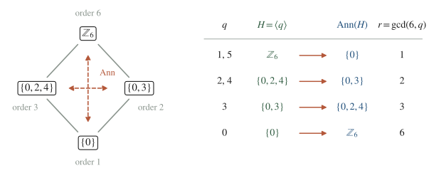
Figure 1. The subgroup lattice of ℤ₆ and the annihilator map. Ann reverses inclusions (it turns the diamond upside down and exchanges the two middle subgroups), |H|·|Ann(H)| = 6, and |Ann(⟨q⟩)| = gcd(6,q).

3.5 What the residual symmetry distinguishes

Charge coprime to $N$ ($r=1$). Every Wilson loop has a perimeter law in every phase (§3.2, Week 13), so the area-law criterion is unavailable; and no element of ${\mathbb{Z}}_N^{(1)}$ keeps a topological operator (3.3), so the symmetry criterion is unavailable too. They fail together because they are one criterion: the area law is the statement that the electric 1-form symmetry is unbroken, and it presupposes an exact symmetry (conventions §6). This is the content of Fradkin–Shenker, and complementarity then says that no transition separates the Higgs and confining regimes (Week 13).

Charge with $r>1$ [Controlled at leading order in the plaquette coefficients; the separation of phases Heuristic]. The loops $W_e$ with $e\notin H$, that is $e\not\equiv 0(\mathrm{mod}r)$, carry charge $e$ mod $r$ under ${\mathbb{Z}}_r^{(1)}$. At small β they have an area law for every κ. In the strong-coupling expansion of (2.2) (§4.2 gives the character expansion) the plaquettes carry charges $k_P\in {\mathbb{Z}}_N$ and the matter supplies lines of charge in $H$; reducing every charge modulo $H$ removes the matter and leaves a ${\mathbb{Z}}_r$ surface bounded by $C$ with the nonzero charge $e$ mod $r$. Every surface therefore contains at least $A(C)$ plaquettes whose charge lies outside $H$, each weighted by a coefficient that vanishes as $\beta \to 0$. At $\kappa =\infty$ and large β the theory (2.3) is deconfined and the same loops have a perimeter law. So ${\mathbb{Z}}_r^{(1)}$ is unbroken in the confined region and spontaneously broken in the deconfined ones, and a transition must separate them. The $\kappa =\infty$ edge exhibits it exactly, at ${\beta }_c({\mathbb{Z}}_r)$. Figure 2 annotates the phase diagram accordingly.

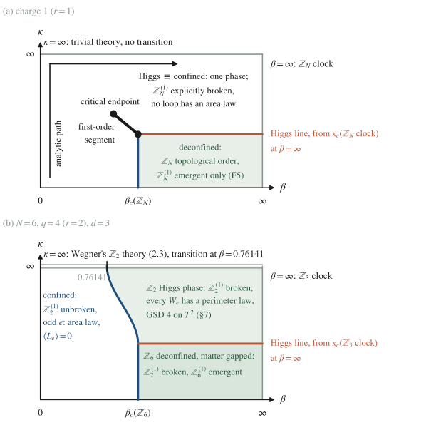
Figure 2. The (β, κ) plane annotated by the realization of the exact electric symmetry (schematic; Week 13’s Figure 1 is the precise diagram for N = 2). (a) With charge-1 matter nothing is exact, the Higgs and confining regimes are joined by an analytic path, and the deconfined region is a separate phase whose distinction is topological order. (b) With charge 4 in ℤ₆ the residual ${\mathbb{Z}}_2^{(1)}$ is exact, unbroken in the confined region and broken in both deconfined regions, so a transition line must separate them; on the κ = ∞ edge it is Wegner’s transition.

Physical picture. Charge-$q$ matter can end any flux line whose charge lies in $H$, so those lines break, while a line of charge $e\notin H$ can only be converted into another line of the same class $e+H$ and never removed. A lattice simulation of the $N=6$, $q=4$ model would therefore see Creutz ratios of $W_2$ and $W_4$ that fall to zero for large loops in every phase, while those of $W_1$ and $W_3$ stay at a finite string tension in the confined region and vanish in the deconfined ones, together with a singularity of the plaquette energy at the boundary; with $q=1$ every Creutz ratio falls to zero and no singularity is required. The exact content is (3.3)–(3.5) and the reduction (2.3); the separation of the phases rests on the SSB criterion of conventions §6. The research line reads the same arithmetic backward: a condensate of charge $k$ leaves the residual symmetry $\mathrm{Ann}(⟨k⟩)\cong {\mathbb{Z}}_{\gcd (N,k)}$, and Semester II Week 14 relates the same arithmetic to subgroup gauging on a hypersurface, the setting of the group’s manuscript in preparation, which the master-project takes up (forward reference; F1).

4. The Polyakov loop and the center symmetry at finite temperature

4.1 The thermal lattice and the center transformation [Proved.]

Make the Euclidean time periodic with $N_{\tau }$ sites, so that $T=1/N_{\tau }$. The Polyakov loop of charge $e$ is

$$L_e(\vec{x})={\omega }^{e{\sum }_{\tau =0}^{N_{\tau }-1}{a}_0(\vec{x},\tau )},L\equiv L_1,$$

the Wilson loop that winds the thermal circle, gauge invariant as every closed loop is; as in Week 6 §7.6 we keep $P$ for plaquettes. Add $s$ to every time-like link $a_0(\vec{x},{\tau }_0)$ of one slice. The shift λ is closed: every $(0,i)$ plaquette of that slice contains two of these links with opposite orientations, and no other plaquette contains any. It is not exact, since its sum around the thermal circle is $s$, while ${\sum }_{\tau }(d\chi {)}_0=0$ around any closed loop. In pure gauge theory the action is invariant and $L_e\to {\omega }^{es}{L}_e$, so

$$⟨L_e⟩={\omega }^{es}⟨L_e⟩,$$

and $⟨L_e⟩=0$ unless the symmetry is spontaneously broken. Restricted to a region $R$ of the slice, the same shift is $U_s(\tilde{c})$ on the closed $(d-2)$-surface $\partial R$ of that slice, which links the Polyakov lines through $R$: the finite-temperature center symmetry is the part of ${\mathbb{Z}}_N^{(1)}$ whose operators lie in one time slice (F3). With charge-$q$ matter the shift leaves (2.1) invariant exactly when $qs\equiv 0$, so for $e\notin H$ the element $s=N^{\prime }$ acts by $e^{2\pi ie/r}\ne 1$ and

$$⟨L_e⟩=e^{2\pi ie/r}⟨L_e⟩,e\notin H,$$

so $⟨L_e⟩=0$ unless the residual ${\mathbb{Z}}_r$ center symmetry is spontaneously broken, and identically in a finite spatial volume (F2), while $⟨L_q⟩\ne 0$ at every coupling (§4.3). Note that nothing here contradicts Elitzur’s theorem. $L_e$ is gauge invariant, and the center transformation acts on the whole spatial slice at once; with a source $h{\sum }_{\vec{x}}\mathrm{Re}L(\vec{x})$ it changes the weight by up to $e^{2h{V}_s}$, which grows with the spatial volume $V_s$, so the limits $h\to 0$ and $V_s\to \infty$ need not commute (Week 5 F1). The expectation value has a thermodynamic meaning. In temporal gauge the time-like links of one slice implement the Gauss-law projector (Week 7 F1); inserting $L(\vec{x})L(\vec{y}{)}^{\ast }$ inserts the characters ${\omega }^{\pm \lambda }$ at $\vec{x}$ and $\vec{y}$ in that projection, which then projects onto states with a static unit charge at $\vec{x}$ and its conjugate at $\vec{y}$. Thus $⟨L(\vec{x})L(\vec{y}{)}^{\ast }⟩=e^{-[F_{q\bar{q}}(r)-F_0]/T}$ and $⟨L⟩=e^{-F_q/T}$: $⟨L⟩=0$ means that an isolated static charge has infinite free energy.

4.2 The correlator at strong coupling [Controlled to leading order in ${\tilde{c}}_1$.]

The character expansion of the ${\mathbb{Z}}_N$ Wilson weight is, in the notation of conventions §4 with $d_r=1$,

$$e^{\beta \cos (2\pi u/N)}=\frac{{\lambda }_0}{N}[1+\sum _{k=1}^{N-1}{\tilde{c}}_k{\omega }^{ku}],{\lambda }_k=\sum _{u=0}^{N-1}{e}^{\beta \cos (2\pi u/N)}{\omega }^{ku},{\tilde{c}}_k=\frac{{\lambda }_k}{{\lambda }_0}={\tilde{c}}_{-k},$$

where the inversion uses ${\sum }_u{\omega }^{(k-k^{\prime })u}=N{\delta }_{k{k}^{\prime }}$. Explicitly, ${\tilde{c}}_1=\tanh \beta$ for $N=2$; ${\tilde{c}}_1=(1-e^{-3\beta /2})/(1+2e^{-3\beta /2})$ for $N=3$; ${\tilde{c}}_1=\tanh (\beta /2)$ and ${\tilde{c}}_2={\tanh }^2(\beta /2)$ for $N=4$; and ${\tilde{c}}_1=\beta /2+O({\beta }^2)$ for every $N\ge 3$ (all checked numerically). Expanding every plaquette assigns a charge $k_P$ to each plaquette with weight ${\tilde{c}}_{k_P}$, and the sum over each link gives $N$ times the constraint that the charges of the plaquettes around it, with the charge of any inserted loop, add up to zero modulo $N$: only closed surfaces survive, or surfaces bounded by the inserted loops (Week 5 §4.1 for $N=2$). For $⟨L(\vec{x})L(\vec{y}{)}^{\ast }⟩$ with $\vec{x}$ and $\vec{y}$ a distance $r$ apart on an axis, the surface must connect the two lines in each of the $N_{\tau }$ slabs between consecutive time slices, which takes at least $r$ time-like plaquettes per slab. The minimum is attained only by the flat strip of Figure 3, with charge 1 on each of its $N_{\tau }r$ plaquettes, whose interior links cancel in pairs. Therefore

$$⟨L(\vec{x})L(\vec{y}{)}^{\ast }⟩={\tilde{c}}_1^{N_{\tau }r}[1+O(N_{\tau }r{\tilde{c}}_1^4)+O(r{\tilde{c}}_1^{2N_{\tau }})],F_{q\bar{q}}(r)-F_0=\sigma r+\dots ,\sigma =-\ln {\tilde{c}}_1,\text{\hspace{1em}(4.1)}$$

with $T{N}_{\tau }=1$. The free energy of the static pair rises linearly, with the zero-temperature string tension at leading order, and $⟨L{L}^{\ast }⟩\to 0=|⟨L⟩{|}^2$ as $r\to \infty$, as cluster decomposition requires. The first corrections come from a cube attached to the strip (area $N_{\tau }r+4$, as in Week 5 §4.2) and, for small $N_{\tau }$, from a tube of $4N_{\tau }$ time-like plaquettes that winds the thermal circle and shares one column with the strip (area $N_{\tau }r+2N_{\tau }$, $2(d-2)$ tubes per column). The tubes are the first place where the temperature enters the tension. Week 6 §7.6 gives the $SU(N)$ version of the leading term.

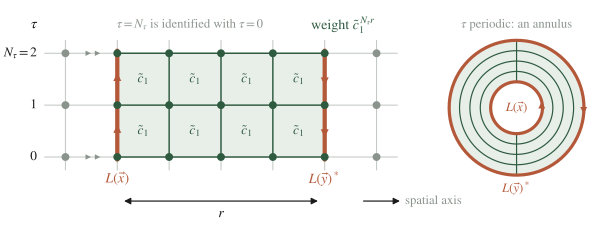
Figure 3. The leading surface of $⟨L(\vec{x})L(\vec{y}{)}^{\ast }⟩$ at strong coupling: the strip of $N_{\tau }r$ time-like plaquettes between the two Polyakov lines (here $N_{\tau }=2$, $r=4$). It is an annulus, since the thermal direction is periodic, and its weight is ${\tilde{c}}_1^{N_{\tau }r}$.

4.3 Charge-$q$ matter: explicit and residual center breaking [Controlled to leading order in $h_1$ and ${\tilde{c}}_k$.]

In unitary gauge the matter enters through the link weight $e^{\kappa \cos (2\pi qa/N)}$, a function of $u=qa\in H$. Writing $u=r{u}^{\prime }$ with $u^{\prime }\in {\mathbb{Z}}_{N^{\prime }}$ and applying the expansion of §4.2 to ${\mathbb{Z}}_{N^{\prime }}$,

$$e^{\kappa \cos (2\pi q{a}_{\ell }/N)}=b_0[1+\sum _{j=1}^{N^{\prime }-1}{h}_j{\omega }^{jq{a}_{\ell }}],h_j={\tilde{c}}_j^{(N^{\prime })}(\kappa ),$$

where $h_1=\tanh \kappa$ for $N^{\prime }=2$ and $h_1=\kappa /2+O({\kappa }^2)$ for $N^{\prime }\ge 3$. The character ${\omega }^{jq{a}_{\ell }}$ is one step of a matter worldline of charge $jq\in H$. Three consequences follow.

• For $e\notin H$, $⟨L_e⟩=0$ unless the residual ${\mathbb{Z}}_r$ center symmetry is spontaneously broken (§4.1), and at strong coupling it is not.
• For $e=q$, the matter worldline that winds the thermal circle at $\vec{x}$ with charge $-q$ (the characters $j=N^{\prime }-1$, of weight $h_{N^{\prime }-1}=h_1$) cancels $L_q(\vec{x})$ on every configuration, so

$$⟨L_q⟩=h_1^{N_{\tau }}[1+\dots ]\ne 0,F_q=-T\ln ⟨L_q⟩=m\equiv -\ln h_1:$$

the center symmetry is broken explicitly, and a static charge $q$ binds one matter quantum of charge $-q$. Complete enumeration for $N=4$, $q=2$, $d=2$, $N_{\tau }=2$ on a ring of three sites gives $⟨L_2⟩/{\tanh }^2\kappa =1.000007$ at $\beta =\kappa =0.05$ and $|⟨L_1⟩|,|⟨L_3⟩|<10^{-15}$.

• For the correlator of $L_q$ the strip (with coefficient ${\tilde{c}}_q$) competes with two dressed lines, $⟨L_q{L}_q^{\ast }⟩\simeq {\tilde{c}}_q^{N_{\tau }r}+h_1^{2N_{\tau }}$, and the string breaks at $r_{\ast }=2\ln h_1/\ln {\tilde{c}}_q$, that is ${\sigma }_q{r}_{\ast }=2m$, independently of $N_{\tau }$ at this order, as at zero temperature (Week 13). For $e\notin H$ the matter can change the charge of the sheet within $e+H$ but never remove it, so $⟨L_e{L}_e^{\ast }⟩$ decays as $e^{-\sigma N_{\tau }r}$ with σ the smallest tension in the class $e+H$.

5. Svetitsky–Yaffe at model level

5.1 The exact reduction at ${\beta }_s=0$ [Computed.]

Give the time-like plaquettes the coupling ${\beta }_t$ and the space-like ones ${\beta }_s$, and set ${\beta }_s=0$ in pure gauge theory. Gauge transformations on the slices $\tau =1,\dots ,N_{\tau }-1$ set $a_0(\vec{x},\tau )=0$ for $\tau \le N_{\tau }-2$; each is a bijection, so $Z=N^{(N_{\tau }-1)V_s}{\sum }_{\mathrm{gauge}\mathrm{fixed}}{e}^{-S}$, and the last time-like link carries the Polyakov-loop phase, $a_0(\vec{x},N_{\tau }-1)={\varphi }_{\vec{x}}$ with $L(\vec{x})={\omega }^{{\varphi }_{\vec{x}}}$. The time-like plaquette at $(\vec{x},\tau )$ in the $(0,i)$ plane has $(da{)}_P=a_0(\vec{x},\tau )+a_i(\vec{x},\tau +1)-a_0(\vec{x}+\hat{i},\tau )-a_i(\vec{x},\tau )$, which in this gauge is $b_{\tau +1}-b_{\tau }$ with $b_{\tau }=a_i(\vec{x},\tau )$, except on the last slab, where it is $b_0-b_{N_{\tau }-1}+\theta$ with $\theta ={\varphi }_{\vec{x}}-{\varphi }_{\vec{x}+\hat{i}}$. With ${\beta }_s=0$ no other plaquette exists, so each spatial link carries an independent periodic chain, coupled to the rest only through θ:

$$Z_{\mathrm{chain}}(\theta )=\sum _{b\in {\mathbb{Z}}_N^{N_{\tau }}}\prod _{\tau =0}^{N_{\tau }-1}w(b_{\tau +1}-b_{\tau }+\theta {\delta }_{\tau ,N_{\tau }-1}),w(u)=e^{{\beta }_t\cos (2\pi u/N)},b_{N_{\tau }}\equiv b_0.$$

Insert $w(u)=N^{-1}{\sum }_k{\lambda }_k{\omega }^{-ku}$ on every bond. Each $b_{\tau }$ appears in two adjacent bonds with opposite signs, so its sum gives $N{\delta }_{k_{\tau -1}{k}_{\tau }}$; all the $k$ are equal, the twist contributes ${\omega }^{-k\theta }$, and with ${\lambda }_k={\lambda }_{-k}$,

$$Z_{\mathrm{chain}}(\theta )=\sum _{k=0}^{N-1}{\lambda }_k^{N_{\tau }}{\omega }^{-k\theta }={\lambda }_0^{N_{\tau }}\sum _{k=0}^{N-1}{\tilde{c}}_k({\beta }_t{)}^{N_{\tau }}{\omega }^{k\theta }.$$

Therefore

$$\boxed{Z=N^{(N_{\tau }-1)V_s}{\lambda }_0^{N_{\tau }(d-1)V_s}\sum _{\varphi \in {\mathbb{Z}}_N^{V_s}}\prod _{(\vec{x},i)}\sum _{k=0}^{N-1}{\tilde{c}}_k({\beta }_t{)}^{N_{\tau }}{\omega }^{k({\varphi }_{\vec{x}}-{\varphi }_{\vec{x}+\hat{i}})},L(\vec{x})={\omega }^{{\varphi }_{\vec{x}}},}\text{\hspace{1em}(5.1)}$$

a $(d-1)$-dimensional nearest-neighbour ${\mathbb{Z}}_N$ spin model for the Polyakov-loop phases, invariant under the global center shift $\varphi \to \varphi +s$. For $N=2$ the bond weight is $1+x{s}_{\vec{x}}{s}_{\vec{y}}\propto e^{K{s}_{\vec{x}}{s}_{\vec{y}}}$ with

$$\tanh K=x=(\tanh {\beta }_t{)}^{N_{\tau }},$$

so the finite-temperature ${\mathbb{Z}}_2$ gauge theory at ${\beta }_s=0$ is the $(d-1)$-dimensional Ising model. Complete enumeration of the $2^{24}$ configurations for $d=3$, $N_{\tau }=2$ on a $2\times 2$ spatial torus at ${\beta }_t=0.6$ gives $⟨LL⟩=0.6326870$ for nearest neighbours and $0.5249808$ across the diagonal, equal to the effective model to $10^{-14}$; the chain formula was checked for $N=2,\dots ,5$ and $N_{\tau }=1,\dots ,4$. Four consequences are exact at ${\beta }_s=0$. (i) In $d=3$ the Polyakov loops order at $(\tanh {\beta }_t{)}^{N_{\tau }}=\tanh K_c=\sqrt{2}-1$ (Week 4, $\sinh 2K_c=1$), which for $N_{\tau }=2$ is ${\beta }_t=0.7643$. (ii) In $d=4$ they order at $(\tanh {\beta }_t{)}^{N_{\tau }}=\tanh K_c=0.2180946$, with $K_c=0.221654626$ the 3d Ising value of conventions §4 (Ferrenberg–Xu–Landau 2018), which for $N_{\tau }=2$ is ${\beta }_t=0.5062$; the exponents are those of the Ising model in $d-1$ dimensions. (iii) In $d=2$, (5.1) is a closed chain, which never orders: two-dimensional gauge theory confines at every temperature, as it confines at every coupling (Week 5 §6). (iv) The leading term of the high-temperature expansion of $⟨{\omega }^{{\varphi }_{\vec{x}}-{\varphi }_{\vec{y}}}⟩$ in (5.1), a path of $r$ bonds of weight ${\tilde{c}}_1^{N_{\tau }}$ each, is the strip (4.1).

5.2 ${\beta }_s>0$ and the universality claim [Stated — refs: Svetitsky–Yaffe 1982.]

For ${\beta }_s>0$ the space-like plaquettes couple neighbouring chains, and integrating out the spatial links gives an effective action for φ with couplings of longer range and with more spins, all invariant under the global ${\mathbb{Z}}_N$. They decay exponentially with distance as long as the spatial links have a finite correlation length at the transition, which holds because the spatial gauge field of the reduced $(d-1)$-dimensional theory confines (F3). The claim of Svetitsky and Yaffe, stated precisely: if the deconfinement transition of a $d$-dimensional gauge theory with center ${\mathbb{Z}}_N$ is continuous, its critical behavior is that of a fixed point of $(d-1)$-dimensional, short-ranged, ${\mathbb{Z}}_N$-symmetric spin models, with the Polyakov loop as the order parameter; where such models have a single fixed point, the exponents are predicted. The argument says nothing about whether the transition is continuous, which is dynamical input. For ${\mathbb{Z}}_2$ and $SU(2)$ in $d=4$ it predicts 3d Ising exponents if the transition is continuous. For center ${\mathbb{Z}}_3$ the Landau–Ginzburg functional of $L$ admits the cubic invariant $\mathrm{Re}{L}^3$, which generically drives the transition first order in three dimensions [Heuristic], and then no universal exponents are predicted. For ${\mathbb{Z}}_4$ in $d=3$, where the spin models are two-dimensional, they form a line of fixed points, the Ashkin–Teller line (Problem 4⋆). With fundamental matter $⟨L⟩\ne 0$ at every temperature (§4.3), and deconfinement is generically a crossover, like a magnet in a field [Heuristic]; with charge $q$ and $r>1$ the loops $L_e$ with $e\notin H$ remain order parameters, and the same reasoning applies with ${\mathbb{Z}}_r$ in place of ${\mathbb{Z}}_N$ [Heuristic; the course’s extension].

6. ‘t Hooft’s flux sectors on the three-torus [Computed.]

6.1 The Hamiltonian and the electric flux

Take a spatial $T^3$ of $L^3$ sites ($d=4$) and put ${\mathbb{C}}^N$ on each link, with $Z_{\ell }|a⟩={\omega }^a|a⟩$, $X_{\ell }|a⟩=|a+1⟩$ and $Z_{\ell }{X}_{\ell }=\omega X_{\ell }{Z}_{\ell }$ (Week 2 §8). With $B_P={\omega }^{(da{)}_P}$, the product of the $Z_{\ell }^{\pm 1}$ around $P$,

$$H=-\Gamma \sum _{\ell }\mathrm{Re}{X}_{\ell }-K\sum _P\mathrm{Re}{B}_P,\mathrm{Re}O\equiv \frac{1}{2}(O+O^{†}),\text{\hspace{1em}(6.1)}$$

which for $N=2$ is the Hamiltonian of conventions §4. The operator $G_x={\prod }_i{X}_{(x-\hat{i},i)}{X}_{(x,i)}^{†}$ implements $a\to a+d{\delta }_x$, and physical states obey $G_x=1$. Define the electric-flux operators

$$U_i(n)=\prod _{x:x_i=n}{X}_{(x,i)},$$

the product over the $i$-links that cross the dual plane $x_i=n+\frac{1}{2}$. Four facts follow. (1) $[U_i(n),H]=0$: $U_i(n)$ commutes with every $X_{\ell }$, and it shifts $a$ by a closed λ (the argument of §4.1), so it commutes with every $B_P$. (2) $U_i$ is topological: in ${\prod }_{x_i=n+1}{G}_x$ the $j$-links of the plane telescope, leaving ${\prod }_{x_i=n+1}{G}_x=U_i(n)U_i(n+1{)}^{†}$, so $U_i(n)=U_i(n+1)\equiv U_i$ on physical states. (3) $U_i^N=1$, and its eigenvalues ${\omega }^{e_i}$ define the electric flux $\vec{e}\in {\mathbb{Z}}_N^3$; in the eigenbasis $X_{\ell }|E⟩={\omega }^E|E⟩$, $U_i={\omega }^{\sum E_{\ell }}$ is the flux through the plane. (4) With $W_j={\prod }_{\ell \in C_j}{Z}_{\ell }$ on a straight noncontractible loop along $j$,

$$W_j{U}_i={\omega }^{{\delta }_{ij}}{U}_i{W}_j,$$

since $C_j$ crosses the plane perpendicular to $i$ once if $i=j$ and shares no link with it otherwise. The three pairs $(W_i,U_i)$ are clock–shift pairs, and the phase is Week 2’s intersection pairing of 1-cycles and 2-cycles on $T^3$.

6.2 Twisted boundary conditions and the magnetic flux

For a closed $n\in C^2(T^3,{\mathbb{Z}}_N)$ let $H[n]$ be (6.1) with $B_P\to {\omega }^{n_P}{B}_P$. For $V_{\lambda }={\prod }_{\ell }{X}_{\ell }^{{\lambda }_{\ell }}$, $V_{\lambda }{B}_P{V}_{\lambda }^{†}={\omega }^{-(d\lambda {)}_P}{B}_P$, and $V_{\lambda }$ commutes with the electric term and with $G_x$, so $H[n]$ and $H[n+d\lambda ]$ are unitarily equivalent. The invariants are the fluxes

$$m_k=\sum _{P\in T_{ij}^2(x_k)}{n}_P(\mathrm{mod}N),(ijk)\text{cyclic},$$

unchanged under $n\to n+d\lambda$ by Stokes and independent of $x_k$ because $dn=0$; two closed $n$ with equal fluxes differ by an exact cochain, since $H^2(T^3,{\mathbb{Z}}_N)\cong {\mathbb{Z}}_N^3$ is detected by the three fluxes (Week 2 §4.3). The sectors are thus labelled by $\vec{m}\in {\mathbb{Z}}_N^3$, with the representative $n_P=m_k$ on the $(ij)$-plaquettes of one column along $k$. Since ${\sum }_{P\in T^2}(da{)}_P=0$ identically, a net magnetic flux through a two-torus exists only as such a twist, which is ‘t Hooft’s twisted boundary condition. $U_i$ and $G_x$ commute with every $H[\vec{m}]$, so $\vec{e}$ is defined in every sector. Inserting $U^{\vec{k}}=U_1^{k_1}{U}_2^{k_2}{U}_3^{k_3}$ in the trace is the temporal twist $n_{0i}=-k_i$ of the Euclidean theory in the convention $B_P\to {\omega }^{n_P}{B}_P$ used here (the symmetry operator of conventions §6 on a spatial dual plane at one time, which replaces $(da{)}_P$ by $(da{)}_P-k_i$), and $\vec{m}$ is the spatial twist $n_{ij}={ϵ}_{ijk}{m}_k$; so $Z[\vec{k},\vec{m}]={\mathrm{tr}}_{\vec{m}}\left(U^{\vec{k}}{e}^{-H[\vec{m}]/T}\right)$. Since ${\sum }_{k=0}^{N-1}{\omega }^{k(e^{\prime }-e)}=N{\delta }_{e{e}^{\prime }}$, the operator $P_{\vec{e}}=N^{-3}{\sum }_{\vec{k}}{\omega }^{-\vec{k}\cdot \vec{e}}{U}^{\vec{k}}$ projects onto $U_i={\omega }^{e_i}$, and

$$\boxed{Z(\vec{e},\vec{m})={\mathrm{tr}}_{\mathcal{H}[\vec{m}]}\left(P_{\vec{e}}{e}^{-H[\vec{m}]/T}\right)=\frac{1}{N^3}\sum _{\vec{k}\in {\mathbb{Z}}_N^3}{\omega }^{-\vec{k}\cdot \vec{e}}Z[\vec{k},\vec{m}],}\text{\hspace{1em}(6.2)}$$

‘t Hooft’s flux partition functions. For a contractible dual loop $\tilde{C}=\partial \tilde{S}$ in space, $T_m(\tilde{C})={\prod }_{\ell \mathrm{pierced}\mathrm{by}\tilde{S}}{X}_{\ell }^m$ is $V_{\lambda }$ with $d\lambda =m$ on the plaquettes dual to $\tilde{C}$: it creates a closed magnetic flux loop along $\tilde{C}$ (Week 5 §8.3), and

$$W_e(C)T_m(\tilde{C})={\omega }^{em\#(C\cap \tilde{S})}{T}_m(\tilde{C})W_e(C)={\omega }^{em\mathrm{Link}(C,\tilde{C})}{T}_m(\tilde{C})W_e(C),$$

‘t Hooft’s commutation relation for ${\mathbb{Z}}_N$. A twist sector is a flux loop that winds the torus and bounds no surface $\tilde{S}$: no operator creates it, and it enters as a boundary condition.

6.3 The flux table at the two soluble points

Deconfined point, $\Gamma =0$. $H$ is diagonal in $|a⟩$, and each $W_i$ now commutes with it. In the untwisted sector the ground states are the flat configurations, one gauge-invariant state per class of $H^1(T^3,{\mathbb{Z}}_N)\cong {\mathbb{Z}}_N^3$ (Week 2 §4.3): $N^3$ states carrying the irreducible representation of the three pairs $(W_i,U_i)$, one in each $\vec{e}$ sector. In a twisted sector each of the $L$ planes $T_{ij}^2(x_k)$ carries flux $m_k$; if $m_k\ne 0$, each needs at least one plaquette with $(da+n{)}_P\ne 0$, which costs at least $K(1-\cos \frac{2\pi }{N})$, and distinct planes share no plaquettes. Therefore

$$E_0(\vec{e},\vec{m})-E_0\ge K(1-\cos \frac{2\pi }{N})L\#\{k:m_k\ne 0\},E_0(\vec{e},\vec{0})=E_0\forall \vec{e},\text{\hspace{1em}(6.3)}$$

with equality for $m_k=\pm 1$, realized by straight flux lines.

Confined point, $K=0$. $H$ is diagonal in the electric basis, with energy $\Gamma (1-\cos \frac{2\pi E_{\ell }}{N})$ per link above $E_0$; Gauss’s law makes the electric field divergence-free, and each of the $L$ dual planes perpendicular to $i$ must carry the flux $e_i$, so

$$E_0(\vec{e},\vec{m})-E_0\ge \Gamma (1-\cos \frac{2\pi }{N})L\#\{i:e_i\ne 0\},\text{independently of }\vec{m}.\text{\hspace{1em}(6.4)}$$

Figure 4 summarizes the two results. As $T\to 0$, $-T\ln [Z(\vec{e},\vec{m})/Z(\vec{0},\vec{0})]\to E_0(\vec{e},\vec{m})-E_0$: in the deconfined phase electric flux is free and magnetic flux costs a tension times $L$ (in ‘t Hooft’s classification, a Higgs phase), and in the confined phase the roles are exchanged.

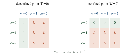
Figure 4. ‘t Hooft’s flux sectors for one direction of the three-torus, N = 3. An entry 0 means that the sector contains a state degenerate with the vacuum at the soluble point; an entry L means that its lowest energy exceeds the vacuum by at least a constant times L, by (6.3) and (6.4). Electric and magnetic flux exchange roles between the two phases; with charge-q matter only e ∈ ${\mathbb{Z}}_N/H$ and m ∈ Ann(H) survive as sector labels (§6.4).

6.4 With charge-$q$ matter

Add the matter clock ${\Phi }_x={\omega }^{{\varphi }_x}$, ${\varphi }_x\in H$, and the shift ${\Pi }_x:{\varphi }_x\to {\varphi }_x+q$:

$$H_q=H-\kappa \sum _{\ell =(x,x+\hat{i})}\mathrm{Re}\left({\Phi }_{x+\hat{i}}{Z}_{\ell }^{-q}{\Phi }_x^{†}\right)-h\sum _x\mathrm{Re}{\Pi }_x,G_x{\Pi }_x=1\text{on physical states},\text{\hspace{1em}(6.5)}$$

the Hamiltonian counterpart of (2.1), with the hopping term invariant under $G_x{\Pi }_x$. For $N=2$, $q=1$ it is the Hamiltonian of Week 13 §9, whose hopping $J$ is written κ here. Now $U_i(n)U_i(n+1{)}^{†}={\prod }_{x_i=n+1}{G}_x={\prod }_{x_i=n+1}{\Pi }_x^{-1}$ on physical states, a product of matter shifts, and $U_i^s(n)U_i^s(n+1{)}^{†}=\prod {\Pi }_x^{-s}=1$ exactly when $qs\equiv 0$. Only $U_i^{N^{\prime }}$, the generator of $\mathrm{Ann}(H)$, stays topological, which is the Hamiltonian form of (3.3), and the electric flux is conserved modulo $H$: $\vec{e}\in ({\mathbb{Z}}_N/H{)}^3$. A twist moves by $V_{\lambda }$ only if $V_{\lambda }$ commutes with the hopping term, $q\lambda \equiv 0$, so only $\vec{m}\in \mathrm{Ann}(H{)}^3$ labels a topological sector; a twist with $qm\not\equiv 0$ is a static flux line that the matter sees through its Aharonov–Bohm phase ${\omega }^{qm}$. The flux sectors thus reduce to $({\mathbb{Z}}_N/H{)}^3\times \mathrm{Ann}(H{)}^3\cong {\mathbb{Z}}_r^3\times {\mathbb{Z}}_r^3$, paired by ${\omega }^{\vec{e}\cdot \vec{m}}$, which is well defined because ${\omega }^{hm}=1$ for $h\in H$ and $m\in \mathrm{Ann}(H)$; at the soluble point of the ${\mathbb{Z}}_r$ Higgs phase, Figure 4 holds with $N\to r$.

7. The deconfined corner: ground-state degeneracy [Computed.]

7.1 The count

Take (6.5) on a spatial $T^2$ at $\Gamma =h=0$ with $K,\kappa >0$. $H_q$ is diagonal in $(a,\varphi )$, and the energy is minimal exactly when $(da{)}_P=0$ on every plaquette and $(d\varphi -qa{)}_{\ell }=0$ on every link. $G_x{\Pi }_x$ acts by permutations, so the gauge-invariant ground states are one per gauge orbit of such configurations. In unitary gauge $\varphi =0$ the conditions become $qa\equiv 0$ and $da=0$: flat connections valued in $\mathrm{Ann}(H)=N^{\prime }{\mathbb{Z}}_N\cong {\mathbb{Z}}_r$, modulo the residual transformations with values in the same subgroup. Therefore

$$\boxed{\mathrm{GSD}(T^2)=|H^1(T^2,{\mathbb{Z}}_r)|=\gcd (N,q{)}^2,}\text{\hspace{1em}(7.1)}$$

and in general $\mathrm{GSD}=r^{b_1}$, with $b_1$ the first Betti number: $r^D$ on a spatial $T^D$, $r^{2g}$ on a surface of genus $g$. The operator form is Week 2 §8. The exact symmetry operators $U_i^{N^{\prime }}$ and the Wilson loops $W_i$ (which commute with $H_q$ at $\Gamma =h=0$ and act on the ground space as ${\mathbb{Z}}_r$ clocks, since ${\omega }^{\sum a}=e^{2\pi i\sum a^{\prime }/r}$ for $a=N^{\prime }{a}^{\prime }$) obey $W_i{U}_i^{N^{\prime }}=e^{2\pi i/r}{U}_i^{N^{\prime }}{W}_i$: two ${\mathbb{Z}}_r$ clock–shift pairs, whose irreducible representation has dimension $r^2$. The checks are $q=1$, one state (Fradkin–Shenker); $q\equiv 0$, $N^2$ states, pure ${\mathbb{Z}}_N$ gauge theory and the toric code for $N=2$ (toric-code; Semester II Week 8); $N=6$, $q=4$, four states. Enumeration on the $2\times 2$ torus gives $\mathrm{GSD}=r^2$ for $(N,q)=(2,0),(2,1),(3,1),(4,0),\dots ,(4,3),(6,0),\dots ,(6,4)$, and the explicit $9\times 9$ and $4\times 4$ matrices of $W_i$ and $U_i^{N^{\prime }}$ on the ground spaces of $(3,0)$ and $(6,4)$ have the stated commutation phases and a commutant consisting of multiples of the identity.

7.2 Away from the soluble point [Sketched.]

The $U_i^{N^{\prime }}$ commute with $H_q$ at every coupling, so the $r^2$ sectors never mix. Their joint eigenvalues label the $r^2$ ground states one by one, so the effective Hamiltonian on the ground space, which commutes with both, is a function of the $U_i^{N^{\prime }}$ alone, and the energies split only through the electric process that generates $U_i^{N^{\prime }}$: the product of $X^{N^{\prime }}$ along a noncontractible dual cycle. A matter loop that winds the torus is $W_{\mp q}$, which equals 1 on the ground space because $qa\equiv 0$ there, and it splits nothing. The electric process takes $N^{\prime }$ steps on each of the $L$ links it crosses, so the splitting appears first at order $N^{\prime }L$ in $\Gamma /K$ and is exponentially small in $L$; on $T^D$ the count is $N^{\prime }{L}^{D-1}$. We omit the degenerate perturbation theory that fixes the prefactor. In the ${\mathbb{Z}}_N$-deconfined region at small κ, with the matter gapped, the $N^2$ states of pure ${\mathbb{Z}}_N$ theory split into $r^2$ exact sectors of $N^{\prime 2}$ states each, mixed by charge-$q$ matter loops that wind the torus: there the degeneracy $N^2$ is topological and approximate, while the $r^2$ sector labels are exact (F5).

8. A superconductor is topologically ordered

8.1 The charge-2 model and its residual ${\mathbb{Z}}_2^{(1)}$ [Proved.]

Hansson, Oganesyan and Sondhi argue that an s-wave superconductor coupled to dynamical electromagnetism is ${\mathbb{Z}}_2$ topologically ordered [Stated — refs: HOS, cond-mat/0404327]. We derive the lattice form. Take the $U(1)$ gauge field $a_{\ell }\in (-\pi ,\pi ]$ of conventions §4 and a Cooper-pair field of fixed modulus (the London limit), ${\varphi }_x\in (-\pi ,\pi ]$, of charge 2:

$$S=-\beta \sum _P\cos (da{)}_P-\kappa \sum _{\ell }\cos (d\varphi -2a{)}_{\ell },\text{\hspace{1em}(8.1)}$$

where the action is invariant under $a\to a+d\lambda$, $\varphi \to \varphi +2\lambda$. The $U(1)$ version of (3.1) shifts $(da{)}_P$ by α on the plaquettes dual to $\tilde{c}$; the change of variables moves the shift into the hopping term as $2\alpha$, which is invisible exactly when $e^{2i\alpha }=1$. The electric $U(1{)}^{(1)}$ of conventions §6 is broken explicitly to ${\mathbb{Z}}_2^{(1)}=\{0,\pi \}$. In the language of (3.5), the screened charges are $H=2\mathbb{Z}\subset \mathbb{Z}$, $\mathrm{Ann}(2\mathbb{Z})=\{\alpha :e^{2i\alpha }=1\}={\mathbb{Z}}_2$, and the sequence is $0\to {\mathbb{Z}}_2\to U(1)\stackrel{\alpha \mapsto 2\alpha }{\to }U(1)\to 0$, since $\widehat{2\mathbb{Z}}\cong U(1)$; the charges modulo screening are $\mathbb{Z}/2\mathbb{Z}$. A probe of charge 1 (an electron) is unscreened, and a Cooper pair is screened.

8.2 The $\kappa =\infty$ edge is Wegner’s model [Computed.]

Unitary gauge $\varphi =0$ uses $\lambda =-\varphi /2$, with residual freedom $\lambda \in \{0,\pi \}$. As $\kappa \to \infty$ the hopping term forces $\cos 2a_{\ell }=1$, so $a_{\ell }\in \{0,\pi \}$, ${\sigma }_{\ell }=e^{i{a}_{\ell }}=\pm 1$ and $\cos (da{)}_P={\sigma }_P$: (8.1) becomes $S=-\beta {\sum }_P{\sigma }_P$, Wegner’s ${\mathbb{Z}}_2$ gauge theory at the same β, which is (2.3) for $U(1)$ with $q=2$. It is deconfined for $\beta >{\beta }_c=0.76141$ in $d=3$, and for β above the self-dual point $0.44069$ in $d=4$, where the transition is first order (conventions §4; Week 5 §9). In the deconfined phase the Hamiltonian ${\mathbb{Z}}_2$ theory at its soluble point has, by (7.1) with $r=2$,

$$\boxed{\mathrm{GSD}=4\text{ on the spatial }{T}^2(2+1\text{ dimensions}),\mathrm{GSD}=8\text{ on the spatial }{T}^3(3+1\text{ dimensions}),}\text{\hspace{1em}(8.2)}$$

split by amounts exponentially small in $L$ away from it (§7.2). The chain is complete: a charge-2 condensate leaves an exact ${\mathbb{Z}}_2^{(1)}$; at $\kappa =\infty$ the theory is Wegner’s; in its deconfined phase ${\mathbb{Z}}_2^{(1)}$ is spontaneously broken and the ground state on the torus is fourfold degenerate. This is the lattice form of “a superconductor is topologically ordered”.

8.3 The dictionary

The ${\mathbb{Z}}_2$ charge is odd electric charge, carried by an unpaired electron; in a BCS superconductor it is a Bogoliubov quasiparticle, whose electric charge is not sharp while its charge modulo 2 is. The ${\mathbb{Z}}_2$ flux, a plaquette with ${\sigma }_P=-1$, is flux π in units where the electron charge is 1, the superconducting flux quantum $h/2e$: a vison in $2+1$ dimensions and a vortex line in $3+1$. The braiding phase of charge 1 around flux π is $e^{i\pi }=-1$ (Week 5 §8.3; conventions §9). The four ground states on $T^2$ are labelled by the holonomies $e^{i\oint a}=\pm 1$ around the two cycles, that is, by whether half a flux quantum $h/2e$ threads each handle. In the flux table of §6, the electric flux modulo 2 is free and a vortex line winding $T^3$ costs its tension times $L$: the Meissner effect in ‘t Hooft’s language.

8.4 What the derivation assumes

The following is the course’s reading of the assumptions [Heuristic], beyond the lattice results of §§8.1–8.2.

1. The gauge field must be dynamical. At $\beta =\infty$, (8.1) is the XY model of Week 1 for φ, which orders by breaking a global $U(1{)}^{(0)}$ and has a gapless Goldstone mode: a neutral superfluid, gapless and without topological order. The exact ${\mathbb{Z}}_2^{(1)}$ and the degeneracy need finite β.
2. What the long-range Coulomb interaction does. The Goldstone mode is removed by the dynamical gauge field (Anderson–Higgs), and it is the Coulomb interaction mediated by $a$ that gaps the phase mode; in a bulk superconductor it lifts the phase mode to the plasma frequency. Every charged excitation must also be gapped, as in an s-wave superconductor.
3. The dimension of electromagnetism. The $2+1$ dimensional count assumes a gauge field in $2+1$ dimensions. A real film couples to the $3+1$ dimensional field outside it, whose Coulomb interaction leaves the in-plane phase mode gapless (the two-dimensional plasmon, $\omega \propto \sqrt{k}$), so the clean statement for real materials is the $3+1$ dimensional one, $\mathrm{GSD}=8$ for a bulk superconductor on $T^3$ with periodic electromagnetism.
4. Finite size. The degeneracy is exact only at the soluble point; in a sample it is split by an amount exponentially small in $L/\xi$, with ξ of the order of the larger of the coherence length and the penetration depth.

Physical picture. An experiment cannot put a superconductor on a torus with periodic electromagnetism, but it sees the ingredients: odd-charge quasiparticles acquire the phase $-1$ around an $h/2e$ vortex, and $h/2e$ flux lines cost a tension, which is the confinement of magnetic flux. What the lattice proves is the chain of §8.2; the physical conditions are the assumptions above. The continuum form of the unit-charge case is the group’s analysis of electric condensation: a BF theory, in which Wilson lines are screened and ‘t Hooft lines confined (Grigorio, Guimaraes, Rougemont, Wotzasek, Zarro, Phys. Rev. D 86 (2012) 027705 [1202.3798]; Guimaraes, Rougemont, Wotzasek, Zarro, Phys. Lett. B 723 (2013) 422 [1209.3073]). A condensate of charge $k$ turns the same construction into a BF theory at level $k$, whose residual data are those of §3 [Stated]; Semester II Week 14 relates such data to subgroup gauging on a hypersurface, the setting of the group’s manuscript in preparation (forward reference).

9. The question the classics leave, answered in part

Against the tempting claim that confinement survives dynamical matter as “the unbroken electric 1-form symmetry”, the statement of the week is the following.

matter	exact electric symmetry	area law at strong coupling for	order parameter at $T>0$	GSD on $T^2$ at the deconfined soluble point
none, or $q\equiv 0$	${\mathbb{Z}}_N^{(1)}$	every $e\ne 0$	$L_e$, $e\ne 0$	$N^2$
charge $q$, $r=\gcd (N,q)>1$	${\mathbb{Z}}_r^{(1)}=\mathrm{Ann}(⟨q⟩)$	$e\notin ⟨q⟩$	$L_e$, $e\notin ⟨q⟩$	$r^2$ (at $\kappa =\infty$)
$q$ coprime to $N$	none	none	none	1 (at $\kappa =\infty$)

With charge-1 matter both criteria fail together, and the Higgs and confining regimes are one phase. The deconfined region at small κ is nonetheless a separate phase: its ${\mathbb{Z}}_N^{(1)}$ is emergent only, and what distinguishes it is topological order, which Semester I sees as the degeneracy at the soluble point and Semester II defines (Weeks 3 and 8; Block 1 and topological-order). With $r>1$ the realization of the exact ${\mathbb{Z}}_r^{(1)}$ separates the confined phase from the deconfined and Higgs phases, and at finite temperature its order parameter is $L_e$ with $e\notin H$. The classics had every operator of this week (Wilson, ‘t Hooft and Polyakov loops, twisted boundary conditions) and knew that the center mattered. What they lacked was the statement that a phase is characterized by the realization of its higher-form symmetries (Gaiotto–Kapustin–Seiberg–Willett; Semester II Week 3) and the identification of the deconfined phases as topologically ordered, which is where Semester II begins (higher-form-symmetries).

10. Subtleties and fine print

F1 — Screening versus gauging. Screening and gauging act on the same exact sequence from opposite ends. Screening by charge-$q$ matter makes the charges in $H$ endable and leaves the subgroup $\mathrm{Ann}(H)$ as the symmetry and the quotient ${\mathbb{Z}}_N/H$ as the line classes modulo screening, with every Wilson loop still genuine. Gauging a subgroup of the symmetry itself, which Semester II Week 4 defines (Block 1; Aharony–Seiberg–Tachikawa), sums over its backgrounds, leaves a quotient of the symmetry group as the residual symmetry and a subgroup of the charges as the genuine lines, and adds a dual symmetry (conventions §6). Through the self-pairing ${\omega }^{se}$ of ${\mathbb{Z}}_N$ both sets of data are ${\mathbb{Z}}_r$, and which operation a given lattice mechanism implements is a question with content. Semester II Week 14 shows that in $2+1$ dimensions a charge-$k$ condensate restricted to a surface reproduces, in its London limit, the condensation sheet of Semester II Week 13, the higher gauging on that surface of the subgroup of the magnetic symmetry generated by the Wilson lines of charge in $⟨k⟩$; it then studies the four-dimensional wall that gauges $⟨k⟩$ within the electric symmetry, the same sequence read on the other side of the pairing, which is the setting of the group’s manuscript in preparation [Stated — forward reference to Semester II Week 14 and the master project].

F2 — Large $N_{\tau }$ versus the continuum limit. The bare Polyakov loop carries the self-energy of a static charge: at fixed lattice spacing its perimeter law gives $⟨L⟩\sim e^{-\mu N_{\tau }}$ even in a deconfined phase, and in a continuum limit at fixed $T$, with $N_{\tau }=1/(T{a}_{\mathrm{lat}})\to \infty$, the bare $⟨L⟩$ vanishes in every phase. Only a renormalized loop $L_R=e^{\mu N_{\tau }}L$, with a scheme-dependent μ, has a limit; whether $⟨L_R⟩$ vanishes, and ratios such as $⟨L(\vec{x})L(\vec{y}{)}^{\ast }⟩/|⟨L⟩{|}^2$, are scheme independent. In a finite spatial volume $⟨L⟩=0$ exactly, and the order parameter is the cluster limit of $⟨L(\vec{x})L(\vec{y}{)}^{\ast }⟩$ or $⟨|\bar{L}|⟩$ with $\bar{L}$ the spatial average.

F3 — Center symmetry at $T=0$ versus $T>0$: temporal versus spatial wrapping. On $S^1\times {\mathbb{R}}^{d-1}$ the electric ${\mathbb{Z}}_N^{(1)}$ splits. Operators on closed $(d-2)$-surfaces inside a time slice act on the lines that wind the thermal circle: in the reduced $(d-1)$-dimensional theory this is a 0-form ${\mathbb{Z}}_N$, and $L$ is a local order parameter. Operators that wind the thermal circle, on $S^1\times \sigma$ with σ a closed $(d-3)$-surface in space, act on spatial Wilson loops, a 1-form symmetry of the reduced theory. Deconfinement breaks the first; the second can stay unbroken. At leading order in ${\beta }_s$ a spatial Wilson loop at fixed time needs at least $A(C)$ space-like plaquettes (project any surface bounded by $C$ onto the spatial slice), so it keeps the area law ${\sigma }_s=-\ln {\tilde{c}}_1({\beta }_s)$ for every ${\beta }_t$, including the deconfined phase of §5.1 [Controlled at leading order in ${\beta }_s$]. At $T=0$ the two parts recombine, and the order parameter is the large Wilson loop of conventions §6.

F4 — What Svetitsky and Yaffe assume. The argument needs a continuous transition, an effective action for $L$ with short-range couplings (all other excitations gapped at $T_c$), and a symmetry of the effective model no larger and no smaller than the center; it predicts exponents only when the corresponding class of spin models has a unique fixed point. It does not predict the order of the transition. At ${\beta }_s=0$ every hypothesis can be checked, which is why §5.1 is the model case.

F5 — Explicit breaking and emergent symmetry. “Explicitly broken” means that the broken elements have no topological operator at any coupling, (3.1). It does not mean that their effects are large: in the deconfined region at small κ, with gapped charge-$q$ matter, the operators $U_s$ with $qs\not\equiv 0$ fail to be topological only through virtual matter loops, and the full ${\mathbb{Z}}_N^{(1)}$ re-emerges at long distances. That is why the deconfined phase with $q=1$ survives as a phase although nothing is exact there: its topological order is robust to small perturbations (Semester II), and its degeneracy is exact only up to terms exponentially small in $L$ (§7.2).

F6 — The target space of the matter field. We took $\varphi \in H$. If instead $\varphi \in {\mathbb{Z}}_N$ with charge $q$, then $\varphi$ mod $H$ is gauge invariant, a neutral ${\mathbb{Z}}_r$ spin, and the model acquires a global ${\mathbb{Z}}_r^{(0)}$ symmetry that orders at large κ. Enumeration on the $2\times 2$ torus then gives $\mathrm{GSD}=r^3$ in place of $r^2$ (8 for $N=6$, $q=4$), the extra factor being ordinary spontaneous breaking of a 0-form symmetry. Such a factor must be separated from topological degeneracy before counting, which is what the choice $\varphi \in H$ does.

F7 — Finite volume and the order of limits for the flux sectors. The inequalities (6.3) and (6.4) hold at the soluble points; inside a phase, the zero entries of Figure 4 become energies exponentially small in $L$ and the $L$ entries become tensions times $L$. ‘t Hooft’s criteria are statements about $F(\vec{e},\vec{m})$ as $L\to \infty$ after $T\to 0$, and on a torus with $L$ comparable to the correlation length no sector assignment is meaningful. On $T^3$ the degeneracy is $N^3$ and on $T^2$ it is $N^2$; the counting is homological, $|H^1|$, and the geometry enters only through the splitting.

11. Common misconceptions

• “Center symmetry is a gauge symmetry, since the center is part of the gauge group.” It is tempting because a constant center-valued gauge transformation is an element of the gauge group. But such a transformation acts trivially ($d\lambda =0$ for constant λ), while the center symmetry adds a closed but non-exact λ, a transformation periodic only up to a center element, and it changes the gauge-invariant Polyakov loop by ${\omega }^{es}$ (§4.1). A transformation that changes a physical expectation value is a global symmetry: here the electric 1-form symmetry, whose finite-temperature part is a 0-form symmetry of the reduced theory.
• ”$⟨L⟩\ne 0$ violates Elitzur’s theorem.” It is tempting because the Polyakov loop is built from link variables and deconfinement looks like the ordering of a gauge field. Elitzur’s theorem forbids expectation values of gauge-variant local operators, through a transformation that touches finitely many source terms. $L$ is gauge invariant and non-local in $d$ dimensions, and the center transformation acts on a whole spatial slice, so its source term changes by an amount that grows with the volume and spontaneous breaking is allowed (§4.1).
• “Confinement is the unbroken electric 1-form symmetry, so it remains a sharp criterion with dynamical matter.” It is tempting because the area law is lost to string breaking while the symmetry language seems to survive. The same matter that breaks the string breaks the symmetry explicitly, (3.3). With $\gcd (N,q)=1$ neither criterion exists, and that is Fradkin–Shenker; with $r>1$ the residual ${\mathbb{Z}}_r^{(1)}$ is a sharp criterion, detected by the loops with $e\notin ⟨q⟩$ (§3.5).
• “The four ground states of a superconductor on a torus are the four values of a broken order parameter.” It is tempting because a superconductor is often described as broken $U(1)$. With dynamical electromagnetism the $U(1)$ acts locally and no local order parameter exists (Week 5 §3); the four states are labelled by ${\mathbb{Z}}_2$ holonomies around the cycles, are exchanged by the operators of the exact ${\mathbb{Z}}_2^{(1)}$, and are not distinguished by any local observable (§§7–8).

12. Historical note

‘t Hooft’s 1978 paper, written in the Hamiltonian formalism of $SU(N)$ gauge theory in temporal gauge on a periodic box, introduced the three tools of §6. He imposed boundary conditions twisted by center elements, whose integers are the magnetic flux $\vec{m}$; he defined the electric flux $\vec{e}$ as the eigenvalue label of the gauge transformations that are periodic only up to a center element; and he used the free energies of the flux sectors, together with a new disorder loop $B(C)$ obeying $A(C)B(C^{\prime })=B(C^{\prime })A(C)e^{2\pi in/N}$ with the Wilson loop $A(C)$, to classify the possible massive phases by which loop has an area law. The Polyakov loop as the order parameter of deconfinement at high temperature came in the same years (Polyakov, Phys. Lett. B 72 (1978) 477; Susskind, Phys. Rev. D 20 (1979) 2610). Svetitsky and Yaffe turned the observation that the Polyakov loop is the order parameter of a global center symmetry into the universality argument of §5, whose lattice model case at vanishing spatial coupling is the reduction (5.1). Fradkin and Shenker’s 1979 paper already distinguished matter by its charge under the center, and the observation that a superconductor’s $h/2e$ vortices and odd charges form a ${\mathbb{Z}}_2$ gauge theory is the content of Hansson, Oganesyan and Sondhi’s 2004 paper. The reading of all of this as the realization theory of higher-form symmetries is Gaiotto, Kapustin, Seiberg and Willett’s (2014).

13. What to take away

1. Charge-$q$ matter leaves the exact electric symmetry ${\mathbb{Z}}_{\gcd (N,q)}^{(1)}=\mathrm{Ann}(⟨q⟩)$ [Proved], organized by $0\to \mathrm{Ann}(H)\to {\mathbb{Z}}_N\to \hat{H}\to 0$; the line classes modulo screening are the dual quotient ${\mathbb{Z}}_N/H$. Physically, matter ends the lines it can screen and is invisible to the symmetry elements that cannot see those lines.
2. With $\gcd (N,q)=1$ both confinement criteria fail together (Fradkin–Shenker); with $r>1$ the residual symmetry separates phases, and the $\kappa =\infty$ edge is exactly ${\mathbb{Z}}_r$ gauge theory, (2.3).
3. The Polyakov loop is the finite-temperature order parameter: $⟨L{L}^{\ast }⟩={\tilde{c}}_1^{N_{\tau }r}$ at strong coupling, $⟨L_e⟩=0$ for $e\notin H$ unless the residual ${\mathbb{Z}}_r$ center symmetry is spontaneously broken, $⟨L_q⟩=h_1^{N_{\tau }}$ with matter; at ${\beta }_s=0$ the theory is a $(d-1)$-dimensional ${\mathbb{Z}}_N$ spin model, Ising for $N=2$ with $\tanh K={\tanh }^{N_{\tau }}{\beta }_t$, the model case of Svetitsky–Yaffe, whose general claim needs a continuous transition.
4. ‘t Hooft’s flux sectors are the clock–shift algebra of the 1-form symmetry on $T^3$: $W_j{U}_i={\omega }^{{\delta }_{ij}}{U}_i{W}_j$, twists labelled by $H^2(T^3,{\mathbb{Z}}_N)$, and (6.2); electric and magnetic flux exchange roles between deconfinement and confinement.
5. The deconfined corner has $\mathrm{GSD}=\gcd (N,q{)}^2$ on $T^2$, and a charge-2 condensate of a dynamical $U(1)$ field is Wegner’s ${\mathbb{Z}}_2$ theory with four ground states on $T^2$ and eight on $T^3$: a superconductor is topologically ordered, under the assumptions of §8.4.

14. Looking ahead: Week 15

Week 15 consolidates Semester I: every duality and criterion of the semester restated as a statement about operators on closed submanifolds, a catalogue of the transitions with no local order parameter, and the take-home final, whose fifth problem is the residual symmetry of §3. Semester II then gives the common thread its name, a symmetry is a topological operator, and this week’s objects become its first examples: the flux sectors are backgrounds and charges (Block 1), the degeneracy (7.1) is topological order, and the arithmetic of §3 returns in Semester II Week 14 with the group’s manuscript.

15. Problem set

Problems 1–3 are the classroom core and are solvable from the note alone; Problems 4⋆ and 5⋆ are self-study consolidation with hints; Problem 6⋆⋆ is a research extension that states what is known, what is explored, the sources and what counts as completion.

Core problems (everyone).

1. The case $N=4$. (Extends §§2–3 and §7.1 to all charges of one group.) For $N=4$ and $q=0,1,2,3$: (a) give $H$, $\mathrm{Ann}(H)$, $\hat{H}$ and the sequence (3.5), and decide in each case whether it splits; (b) give the line classes modulo screening and the Wilson loops that can serve as order parameters; (c) identify the theories on the $\kappa =\infty$ and $\beta =\infty$ edges; (d) give the ground-state degeneracy at the soluble point of §7.1 on the spatial $T^2$ and on the closed surface of genus 2; (e) explain why $q=1$ and $q=3$ give identical answers, and why for $q=2$ the residual symmetry and the screened charges are the same subset of ${\mathbb{Z}}_4$; say what this coincidence hides.

2. Polyakov loops with charge-2 matter in ${\mathbb{Z}}_4$. (Extends §§4.2–4.3 to a case where the residual symmetry and explicit breaking coexist.) (a) Show that $⟨L_1⟩=⟨L_3⟩=0$ in a finite spatial volume at every coupling and temperature, and in infinite volume wherever the residual ${\mathbb{Z}}_2$ center symmetry is unbroken, strong coupling included; find $⟨L_2⟩$ at leading order. (b) Compute ${\tilde{c}}_1$ and ${\tilde{c}}_2$ for the ${\mathbb{Z}}_4$ Wilson action and $h_1$ for the matter; find the leading behavior of $⟨L_e(\vec{x})L_e(\vec{y}{)}^{\ast }⟩$ for $e=1,2$ at small β and κ, the breaking distance for $e=2$, and its value at $\beta =1$, $\kappa =0.1$. (c) Explain, in terms of which flux sheets charge-2 matter can end, why $F_1(r)$ keeps rising linearly while $F_2(r)$ saturates.

3. The ‘t Hooft spectrum with charge-$q$ matter. (Extends §§3.1 and 6.4 from Wilson to ‘t Hooft operators.) A ‘t Hooft operator of magnetic charge $m\in {\mathbb{Z}}_N$ shifts $(da{)}_P$ by $m$ on the plaquettes dual to an open dual $(d-2)$-chain $\tilde{\Sigma }$, its Dirac sheet, and lives on $\partial \tilde{\Sigma }$ (Week 5 §8.2). (a) Show that the sheet can be moved to any ${\tilde{\Sigma }}^{\prime }$ with the same boundary without changing the weight of any configuration of the gauge and matter fields if and only if $qm\equiv 0(\mathrm{mod}N)$, so that for these $m$ the sheet is an open operator $U_m$ of the residual symmetry, and identify these magnetic charges. (b) Show that the phase ${\omega }^{em}$ with which such a ‘t Hooft operator detects a linked Wilson loop depends only on the class of $e$ in ${\mathbb{Z}}_N/H$, that the resulting pairing of electric charges modulo screening with these magnetic charges is perfect, and that the operator is therefore not genuine in the sense of §3.2. (c) For $N=6$, $q=4$ list both sets and the phases. (d) In $2+1$ dimensions at the soluble point of §7.1, compare the number of pairs (electric class, magnetic charge in $\mathrm{Ann}(H)$) with $\mathrm{GSD}(T^2)$; what is the degeneracy on the spatial $T^3$ in $3+1$ dimensions?

Starred problems (Ph.D. expected; ambitious M.Sc. encouraged).

4⋆. Svetitsky–Yaffe in $2+1$ dimensions. (a) For $N=3$ at ${\beta }_s=0$, show that (5.1) is the three-state Potts model on the square lattice with $e^K=(1+2x)/(1-x)$, $x={\tilde{c}}_1({\beta }_t{)}^{N_{\tau }}$, and locate the transition at $x_c=(\sqrt{3}-1)/2$ from the self-duality $(e^K-1)(e^{K^{\ast }}-1)=3$; find ${\beta }_{t,c}$ for $N_{\tau }=2$. (b) For $N=4$, show that the bond weight of (5.1) becomes $(1+x{s}_1{s}_1^{\prime })(1+x{s}_2{s}_2^{\prime })$ with $x={\tanh }^{N_{\tau }}({\beta }_t/2)$ under the bijection ${\omega }^{\varphi }=e^{-i\pi /4}(s_1+i{s}_2)/\sqrt{2}$: two decoupled Ising models. Show that the ${\mathbb{Z}}_4$ symmetry allows the coupling $s_1{s}_1^{\prime }{s}_2{s}_2^{\prime }$, argue that ${\beta }_s>0$ generates it, and decide what “the universality class of the ${\mathbb{Z}}_4$ spin model” means. Hint: derive the Potts self-duality by the Kramers–Wannier argument of Week 4 with ${\mathbb{Z}}_3$ variables; for (b), the two Ising models with the four-spin coupling form the Ashkin–Teller model, whose critical exponents vary continuously with that coupling.

5⋆. The superconductor in $3+1$ dimensions. For (8.1) in $d=4$: (a) identify the $\kappa =\infty$ theory and its transition; (b) at the deconfined soluble point give the degeneracy on $T^3$ and the flux table of Figure 4 for $N=2$; (c) translate each entry into superconductor language (electric flux modulo 2, $h/2e$ vortex lines winding the torus, line tension); (d) compute the ‘t Hooft loop of the ${\mathbb{Z}}_2$ theory at weak coupling and interpret its area law as the tension of $h/2e$ flux lines. Hint: Week 5 §§8.2–8.3 give the four-dimensional ‘t Hooft loop at both couplings and the self-dual point; compare the group’s analysis of magnetic confinement in the electric condensate, Phys. Lett. B 723 (2013) 422.

⋆⋆ problems (research extension; optional).

6⋆⋆. The screening data of a charge-$k$ condensate, assembled for the comparison with gauging. What is known. For charge-$k$ matter in ${\mathbb{Z}}_N$ gauge theory, §§3 and 6.4, Problem 3 and (7.1) give the residual symmetry $\mathrm{Ann}(H_k)$, the Wilson classes modulo screening ${\mathbb{Z}}_N/H_k$, the broken part ${\hat{H}}_k$, the ‘t Hooft charges whose sheet is topological, and the degeneracy $r^2$ at the soluble point. What is explored. The same data at finite coupling, organized so that they can be compared with the gauging of $H_k^{(1)}$ once Semester II Week 4 defines it, and with the higher-gauging walls of Semester II Week 14. (a) Tabulate every item above for $(N,k)=(4,2),(6,2),(6,3),(6,4),(8,6),(12,8)$. (b) Diagonalize (6.5) in $2+1$ dimensions for $(N,k)=(4,2)$ on the $2\times 2$ and $3\times 2$ tori at large $K$ and κ and small Γ and $h$, and show that four states separate from the rest with a splitting that decreases with the size. (c) Write one paragraph listing which of the data a gauging of $H_k$ must reproduce, which it adds (the dual symmetry and its operators), and where subgroup and quotient exchange roles (F1). Sources: this note; Week 5; the master-project (its second phase); Block 1 (Week 4) and Block 5 (Week 14). Completion: the table with every entry derived; the diagonalization at two sizes with the trend of the splitting; the paragraph, with every claim labelled as derived here or as a forward reference.

Self-study answer checkpoints

These checkpoints cover the core problems; starred and ⋆⋆ problems remain source-led.

1. The case $N=4$. The decisive step is $H=⟨\gcd (4,q)⟩$ and $\mathrm{Ann}(H)=\{s:qs\equiv 0\}$. For $q=0$: $H=\{0\}$, $\mathrm{Ann}(H)={\mathbb{Z}}_4$, $\hat{H}$ trivial, $0\to {\mathbb{Z}}_4\to {\mathbb{Z}}_4\to 0$; no nonzero charge is screened; the matter disappears and both edges are pure ${\mathbb{Z}}_4$ gauge theory (trivially at $\beta =\infty$); $\mathrm{GSD}=16$ on $T^2$ and $4^4=256$ on genus 2. For $q=1,3$: $H={\mathbb{Z}}_4$, $\mathrm{Ann}(H)=0$, ${\mathrm{res}}_H$ an isomorphism; one class, no order parameter; the $\kappa =\infty$ edge is trivial and the $\beta =\infty$ edge is the ${\mathbb{Z}}_4$ clock model; $\mathrm{GSD}=1$. For $q=2$: $H=\mathrm{Ann}(H)=\{0,2\}$, $\hat{H}\cong {\mathbb{Z}}_2$, and $0\to {\mathbb{Z}}_2\to {\mathbb{Z}}_4\to {\mathbb{Z}}_2\to 0$ does not split, since ${\mathbb{Z}}_4$ has a single element of order 2 and is not ${\mathbb{Z}}_2\times {\mathbb{Z}}_2$; the classes are the parity of $e$ and $W_1$, $W_3$ are the order parameters; at $\kappa =\infty$, $a\in \{0,2\}$ and (2.3) is Wegner’s theory at β; at $\beta =\infty$, $\varphi \in \{0,2\}$ gives the Ising model at κ; $\mathrm{GSD}=4$ on $T^2$ and $2^4=16$ on genus 2. (e) Since 3 is a unit modulo 4, $⟨3⟩=⟨1⟩$: the data depend on $q$ only through $⟨q⟩$ (charge conjugation maps $q\to -q$). For $q=2$, $N^{\prime }=r=2$, so $H=r{\mathbb{Z}}_4$ and $\mathrm{Ann}(H)=N^{\prime }{\mathbb{Z}}_4$ coincide; the coincidence hides that one set consists of symmetry elements (the element 2 acts on $W_1$ as $-1$) and the other of charges (the charge 2 is endable). Common failure mode: concluding from $N=4$ that $H$ and $\mathrm{Ann}(H)$ always coincide, which $N=6$, $q=4$ refutes ($\{0,2,4\}$ against $\{0,3\}$).
2. Polyakov loops in ${\mathbb{Z}}_4$. The decisive step is the action of $s=2\in \mathrm{Ann}(H)$, ${\omega }^{2e}=(-1{)}^e$ on $L_e$, which forces $⟨L_1⟩=⟨L_3⟩=0$ in finite volume, and in infinite volume unless the residual ${\mathbb{Z}}_2$ breaks spontaneously (at $\kappa =\infty$ the model is Wegner’s theory, whose Polyakov loops do order at high temperature), while leaving $L_2$ unconstrained; the matter takes values in $\{0,2\}$ with weights $e^{\pm \kappa }$, so $h_1=\tanh \kappa$ and $⟨L_2⟩={\tanh }^{N_{\tau }}\kappa [1+\dots ]$ (enumeration: ratio $1.000007$ at $\beta =\kappa =0.05$, $N_{\tau }=2$). From ${\lambda }_0=e^{\beta }+2+e^{-\beta }$, ${\lambda }_1=e^{\beta }-e^{-\beta }$ and ${\lambda }_2=e^{\beta }-2+e^{-\beta }$, $${\tilde{c}}_1=\tanh \frac{\beta }{2},{\tilde{c}}_2={\tanh }^2\frac{\beta }{2}.$$ For $e=1$, $⟨L_1{L}_1^{\ast }⟩\simeq {\tanh }^{N_{\tau }r}(\beta /2)$ at every $r$: the matter can turn the charge-1 sheet into a charge-3 sheet, of equal weight since ${\tilde{c}}_3={\tilde{c}}_1$, but cannot remove it, and $F_1={\sigma }_{1}r$ with ${\sigma }_1=-\ln \tanh (\beta /2)$. For $e=2$, $⟨L_2{L}_2^{\ast }⟩\simeq {\tanh }^{2N_{\tau }r}(\beta /2)+{\tanh }^{2N_{\tau }}\kappa$, and the terms cross at $r_{\ast }=\ln \tanh \kappa /\ln \tanh (\beta /2)$, independent of $N_{\tau }$; at $\beta =1$, $\kappa =0.1$, $r_{\ast }=(-2.3059)/(-0.7719)=2.99$. Common failure mode: weighting the charge-2 strip with ${\tilde{c}}_1^{N_{\tau }r}$, which halves ${\sigma }_2$ and doubles $r_{\ast }$, or carrying over the fundamental-matter picture and writing $⟨L_1⟩\propto h_1^{N_{\tau }}$.
3. The ‘t Hooft spectrum. The decisive step is that moving the sheet from $\tilde{\Sigma }$ to ${\tilde{\Sigma }}^{\prime }$ is the change of variables $a\to a-\lambda$ with $\lambda =m$ on the links dual to the $(d-1)$-chain swept between them; by (3.1), with $s\to m$, the hopping term acquires $qm$ on those links, so the sheet is invisible exactly when $qm\equiv 0$, that is $m\in \mathrm{Ann}(H)=N^{\prime }{\mathbb{Z}}_N\cong {\mathbb{Z}}_r$. For other $m$ the swept region carries the matter twist, the sheet is physical and the operator is attached to a surface. (b) Replacing $e$ by $e+h$ multiplies ${\omega }^{em}$ by ${\omega }^{hm}=1$ for $m\in \mathrm{Ann}(H)$; with $m=N^{\prime }{m}^{\prime }$ the pairing is $e^{2\pi i{m}^{\prime }e/r}$, the perfect pairing of ${\mathbb{Z}}_r$. (c) Magnetic charges $\{0,3\}$, electric classes $\{\text{even},\text{odd}\}$, phases ${\omega }^{3e}=(-1{)}^e$. (d) $r^2=4$ pairs, equal to $\mathrm{GSD}(T^2)=r^2$; on $T^3$, $\mathrm{GSD}=|H^1(T^3,{\mathbb{Z}}_r)|=r^3=8$. Common failure mode: testing the invisibility of the sheet against the gauge field alone, which admits every $m$ as in pure gauge theory, or listing the quotient ${\mathbb{Z}}_N/H$ as the magnetic charges.

---

Notes prepared for the generalized-symmetries course, Semester I Block D. Rewritten to the note-quality-template standard on 2026-09-28 (first draft 2026-07-01). Last revised 2026-10-04.