Week 3 — The Villain Form and the Exact Duality of the XY Model

Last week promised that “the vortices are a Coulomb gas.” This week we prove it — exactly, with the sums performed on the page. The route runs through four exact rewritings: the Villain model becomes a conserved-current model, the current model becomes a height model, the height model splits into spin waves plus integer charges, and the charges interact by the two-dimensional Coulomb law, with a fugacity set by the lattice Green function constant of Week 1. Each of these rewritings is an identity. The only expansion of the week comes at the end, when the same partition function is written as a sine-Gordon theory to second order in the fugacity, and that fourth form hands Week 4 the one number it needs: the scaling dimension $\pi \beta$ of the vortex operator.

How to use this chapter

• In class: derive the chain at the board in the order of the note: the vorticity $v=dn$ and its sign (§1.2), Moves 1–3 to the conserved currents (§2), the integer Hodge solution with its tilt sectors (§3, Figure 2), and Moves 4–7 to the neutral Coulomb gas with coefficient $2{\pi }^2\beta$ and $E_{\mathrm{core}}=2{\pi }^2\beta \kappa$ (§4). Take Move 5 slowly: the zero mode runs over one period and brings the Jacobian $\sqrt{N^{\ast }}$. Then state the sine-Gordon form and the vortex dimension $\pi \beta$ (§6), and close with the exact correlator $e^{-a(x-y)/\beta }$ of §7, the reproducible calculation of the week. The core Problems 1–3 extend §7, §§2–4 and §§6–7.
• For self-study: the Hodge proof of §5, the operator table of §6.1, the dictionary of §8 with Figure 3, and the fine print of §9. The one calculation to do alone is §5: rederive $\Vert \delta \xi {\Vert }^2=4{\pi }^2⟨v,G^{\prime }v⟩$ from the Hodge split of $2\pi n$, and check at $v=0$ that the prefactors of the two exact routes agree, which is where the $\sqrt{N^{\ast }}$ of Move 5 is needed.
• Instructor checkpoint: a twist α of the boundary conditions enters as the phase $e^{i\alpha w_1}$ on each tilt sector, and it becomes a shift only after Poisson resummation to the θ-winding variable (F3); shifting $w_1$ itself gives an exponentially small stiffness in place of ${\rm Y}=\beta$. And κ is counted exactly once: with bare vertex operators and the exact kernel the sine-Gordon coupling is $2\cos \chi$ and $y$ comes out of $a(r)$, while with vertices normal-ordered at the lattice scale it is $2y\cos \chi$ (§6); combining $y$ with bare vertices counts the core energy twice (F5).

0. Reading

Primary: José, Kadanoff, Kirkpatrick, Nelson, Phys. Rev. B 16 (1977) 1217 (JKKN), §§I–III — this week reproduces and modernizes their derivation. Villain, J. Physique 36 (1975) 581, for the original substitution.

Secondary:

• Kogut, Rev. Mod. Phys. 51 (1979) 659, §VI — the duality in review form.
• Tong, Statistical Field Theory, §5.3 — Coulomb gas and sine-Gordon in continuum notation.

Optional research reading: Fröhlich & Spencer, Comm. Math. Phys. 81 (1981) 527 — the rigorous proof that the BKT transition exists, built exactly on this week’s Coulomb-gas representation.

Proof-status labels as in Week 1. Cochain machinery: Week 2 and the survival kit; conventions: conventions.

1. The Villain substitution

1.1 The action

The cosine weight $e^{\beta \cos \varphi }$ is $2\pi$-periodic but algebraically opaque: its character coefficients are Bessel functions (Week 1 §5). Villain’s move: keep the periodicity, make each branch Gaussian,

$$e^{\beta \cos \varphi }⟶V_{\beta }(\varphi )=\sum _{n\in \mathbb{Z}}{e}^{-\frac{\beta }{2}(\varphi -2\pi n{)}^2}.$$

On the lattice, $\varphi \to (d\theta {)}_{\ell }={\theta }_y-{\theta }_x$ per link, each link carrying its own integer $n_{\ell }$. The Villain XY partition function is

$$\boxed{Z=\left(\prod _x{\int }_{-\pi }^{\pi }\frac{d{\theta }_x}{2\pi }\right)\sum _{n\in C^1(\Lambda ,\mathbb{Z})}\exp (-\frac{\beta }{2}\Vert d\theta -2\pi n{\Vert }^2),}$$

with $\Vert f{\Vert }^2={\sum }_{\ell }{f}_{\ell }^2$. The integer 1-cochain $n$ is precisely the “pair of ($\mathbb{R}$-cochain, $\mathbb{Z}$-cochain)” that Week 2’s fine print F6 said a compact field really is: $n_{\ell }$ records which branch of the angle difference each link sits on.

We take the Villain model as the definition of the theory this week. Its relation to the cosine model — same universality class, different vortex core energy — is quantified in §9 (F2) and Week 1 Problem 5.

1.2 The branch redundancy and the vorticity [Computed.]

The pair $(\theta ,n)$ overcounts configurations: shifting

$${\theta }_x\to {\theta }_x+2\pi k_x,n\to n+dk,k\in C^0(\Lambda ,\mathbb{Z})$$

changes $d\theta -2\pi n$ by $2\pi dk-2\pi dk=0$. (Equivalently: extending each ${\theta }_x$ integral from $(-\pi ,\pi ]$ to $\mathbb{R}$ while dropping one integer sum is the same partition function.) The branch-independent content of $n$ is its coboundary,

$$v=dn\in C^2(\Lambda ,\mathbb{Z}),$$

one integer per plaquette, invariant under $n\to n+dk$ since $d^2=0$. This is the vorticity: applying $d$ to the Villain field strength,

$$d(d\theta -2\pi n)=-2\pi dn=-2\pi v,$$

so the branch-reduced angle winds by $-2\pi v_P$ around a plaquette $P$, and a counter-clockwise $+2\pi$ vortex, such as the explicit one of Week 1 §4.1, has $v_P=-1$ (the sign is pinned in conventions §4). Week 1’s vortex is now one line of cochain algebra. Section 5 shows, by an exact lattice computation, that these integers carry the Coulomb gas that §4 derives from the dual variables.

Physical picture. The split ”$n$ = branch junk + vorticity” is the split “spin waves + vortices.” The part $dk$ is unwound by letting θ roam $\mathbb{R}$; the part with $dn\ne 0$ cannot be unwound — it is the topological obstruction, and it is all that survives of $n$ in any physical answer. Week 1’s move “let $\theta \in \mathbb{R}$ to get the Gaussian model” is precisely: keep the junk, discard $v$. This week keeps both.

1.3 A vortex pair, walked through the variables [Computed.]

Concreteness before machinery. Take the vortex–antivortex pair of Week 1 §4.3: the phase field $\theta (x)$ winds $+2\pi$ around core plaquette ${\tilde{x}}_1$ and $-2\pi$ around ${\tilde{x}}_2$. Where do the integers sit? The multivalued angle has a branch cut: a curve joining the two cores across which θ jumps by $2\pi$. On the lattice, choose the cut as a path $\tilde{\gamma }$ on the dual lattice from ${\tilde{x}}_2$ to ${\tilde{x}}_1$. On every link crossed by $\tilde{\gamma }$, the branch-reduced difference $(d\theta {)}_{\ell }$ overshoots the fundamental domain, and minimizing the Villain action assigns exactly

$$n_{\ell }=\{\begin{array}{ll}\pm 1& \ell \text{ crossed by }\tilde{\gamma }\\ 0& \text{otherwise}\end{array}\text{i.e.}n=\star 1_{\tilde{\gamma }},$$

the indicator cochain of a string (Figure 0). Its coboundary is supported where the string ends: $dn$ at a plaquette $P$ equals the number of times $\tilde{\gamma }$ leaves the dual site $\tilde{P}$ minus the number of times it arrives there (the out-minus-in rule of §5.2 of Week 2, with Λ and ${\Lambda }^{\ast }$ exchanged: $d$ on Λ ↔ minus the boundary on ${\Lambda }^{\ast }$), so

$$v=dn=+1_{{\tilde{x}}_2}-1_{{\tilde{x}}_1}:$$

the charges live at the string’s ends and nowhere else.

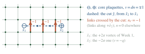
Figure 0. The Villain integer as a Dirac string: $n=\star 1_{\tilde{\gamma }}$ is the indicator of an unobservable cut, transported to the links it crosses; $v=dn$ marks its observable endpoints. The symbols label $v$; since $v=-q$ for a vortex of winding $2\pi q$ (conventions §4), ⊖ is the $+2\pi$ vortex drawn as ⊕ in Week 1’s Figure 2.

Moving the cut, $\tilde{\gamma }\to {\tilde{\gamma }}^{\prime }$ with the same endpoints, changes $n$ by a gauge shift $dk$, with $k=\pm$ the indicator of the sites enclosed between the two cuts: this is §1.2’s redundancy, now with a picture. The string is unobservable; the endpoints are not. Note that the configuration of Figure 0 returns, point for point, as the Dirac string of a magnetic monopole pair (Week 8, Week 12’s Witten effect) and as the seam of the Kadanoff–Ceva disorder operator (Week 4).

2. First rewriting: the conserved-current model [Computed.]

We now execute the Week-2 recipe with every constant. Three moves.

Move 1 — Hubbard–Stratonovich, link by link. For each link, with $u_{\ell }=(d\theta -2\pi n{)}_{\ell }$,

$$e^{-\frac{\beta }{2}{u}_{\ell }^2}=\frac{1}{\sqrt{2\pi \beta }}{\int }_{-\infty }^{\infty }d{b}_{\ell }{e}^{-\frac{1}{2\beta }{b}_{\ell }^2+i{b}_{\ell }{u}_{\ell }}$$

(a Gaussian integral, verified by completing the square). The coupling has already inverted, $\beta \to 1/\beta$ — the fingerprint of duality. Doing all links:

$$Z=(2\pi \beta {)}^{-N_{\ell }/2}\left(\prod _x\int \frac{d{\theta }_x}{2\pi }\right)\left(\prod _{\ell }\int d{b}_{\ell }\right)\sum _n{e}^{-\frac{1}{2\beta }\Vert b{\Vert }^2+ib\cdot (d\theta -2\pi n)},$$

with $N_{\ell }$ the number of links and $b\cdot f={\sum }_{\ell }{b}_{\ell }{f}_{\ell }$.

Move 2 — sum the integers: the comb. The $n$-dependence is ${\prod }_{\ell }{\sum }_{n_{\ell }}{e}^{-2\pi i{b}_{\ell }{n}_{\ell }}$. By the Dirac-comb identity (Week 2 §7.1),

$$\sum _{n_{\ell }\in \mathbb{Z}}{e}^{-2\pi i{b}_{\ell }{n}_{\ell }}=\sum _{m_{\ell }\in \mathbb{Z}}\delta (b_{\ell }-m_{\ell }):$$

the auxiliary field is pinned to integer values, $b=m\in C^1(\Lambda ,\mathbb{Z})$. The $b$ integrals collapse:

$$Z=(2\pi \beta {)}^{-N_{\ell }/2}\left(\prod _x{\int }_{-\pi }^{\pi }\frac{d{\theta }_x}{2\pi }\right)\sum _{m\in C^1(\Lambda ,\mathbb{Z})}{e}^{-\frac{1}{2\beta }\Vert m{\Vert }^2+im\cdot d\theta }.$$

Move 3 — integrate the compact phase: a Kronecker delta. Summation by parts (Week 2 §3.3, the definition of the adjoint):

$$m\cdot d\theta =(\delta m)\cdot \theta =\sum _x(\delta m{)}_x{\theta }_x.$$

Because $m$ is integer-valued, so is $(\delta m{)}_x$, and the compact integral gives a Kronecker — not Dirac — delta:

$${\int }_{-\pi }^{\pi }\frac{d{\theta }_x}{2\pi }{e}^{i(\delta m{)}_x{\theta }_x}={\delta }_{(\delta m{)}_x,0}.$$

This is worth pausing on: compactness of θ is exactly what makes the dual current conserved with integer precision. A noncompact θ would force $\delta m=0$ as a real constraint on a real field; the compact θ forces it on an integer field — the difference between a gauge fixing and a conservation law. The result of the three moves:

$$\boxed{Z=(2\pi \beta {)}^{-N_{\ell }/2}\sum _{\begin{array}{c}m\in C^1(\Lambda ,\mathbb{Z})\\ \delta m=0\end{array}}{e}^{-\frac{1}{2\beta }\Vert m{\Vert }^2}.}$$

The XY model is exactly a statistical mechanics of conserved integer currents on links: divergence-free loops of integer flux with weight $e^{-\Vert m{\Vert }^2/2\beta }$, which for a loop of unit flux is $e^{-(\text{length})/2\beta }$. High-temperature physics (small β) suppresses currents entirely; low temperature lets them proliferate. (This is also precisely the form in which the model’s global $U(1)$ charge sectors are manifest — each closed current loop is a worldline of charge.)

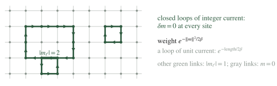
Figure 1. The conserved-current representation: the XY model as a gas of oriented integer loops.

Physical picture. The loops of Figure 1 are worldlines of the $U(1)$ charge: the current representation is what a particle physicist would call the world-line expansion of the theory, with $m_{\ell }$ counting net charge flow through each link. High temperature (small β) suppresses all flow — an insulator of charge; low temperature lets long loops proliferate — the QLRO phase is a loop condensate. This representation is also, verbatim, what Monte Carlo “worm algorithms” simulate, and its gauge-theory sibling — electric flux lines as the dual variable — is the strong-coupling picture of Week 6 and the string-net condensate of Semester II.

3. Second rewriting: heights and windings [Computed.]

Solving $\delta m=0$ is Week 2’s Hodge theory, over the integers, on the torus.

Claim. Every divergence-free $m\in C^1(\Lambda ,\mathbb{Z})$ on the $L\times L$ torus can be written uniquely as

$$m=\star d\tilde{h}+w_1{M}^{(1)}+w_2{M}^{(2)},\tilde{h}\in C^0({\Lambda }^{\ast },\mathbb{Z})\text{(mod global shift)},w_{1,2}\in \mathbb{Z},$$

where $\tilde{h}$ is an integer height field on dual sites and $M^{(1,2)}$ are two fixed reference currents of unit winding — e.g. $M^{(1)}$ is a single closed loop of current along one chosen row of $x$-links. (Note what the $M^{(i)}$ are not: they are not the harmonic cochains $h^{(i)}$ of Week 2 §6, which have value 1 on every parallel link and therefore carry winding $L$, not 1. Over the integers there is no harmonic representative of unit winding — the real harmonic one would be $h^{(i)}/L$, which is not integer-valued. This distinction matters below.)

Construction (this is the proof). Transport $m$ to the dual lattice: $\star m$ is a closed integer 1-cochain on ${\Lambda }^{\ast }$ (§5.2 of Week 2: divergence becomes curl). Measure its two winding numbers $w_i$, the sums of $\star m$ along the two dual cycles, and subtract $w_1{M}^{(1)}+w_2{M}^{(2)}$, whose windings are $(1,0)$ and $(0,1)$ by construction: the remainder $r$ is closed with zero winding. Now define $\tilde{h}(\tilde{x})=-{\sum }_{\gamma :{\tilde{x}}_0\to \tilde{x}}\star r$ along any dual path γ: path-independence holds because two paths differ by a closed dual loop, on which a closed zero-winding cochain sums to zero. So $d\tilde{h}=-\star r$, and since $\star \star =-1$ on 1-cochains in $d=2$ (conventions §2), $r=\star d\tilde{h}$ with $\tilde{h}$ integer-valued, unique up to the constant $\tilde{h}({\tilde{x}}_0)$. $\square$

Equivalently and more usefully: $m=\star d\tilde{h}$ with a multivalued height, $\tilde{h}$ shifting by $w_i$ around the $i$-th cycle — “tilted” or twisted boundary conditions, the lattice version of a screw dislocation. The partition function splits exactly as a sum over tilt sectors,

$$Z=(2\pi \beta {)}^{-N_{\ell }/2}\sum _{w_1,w_2\in \mathbb{Z}}{Z}_{\mathrm{SOS}}^{(w)},Z_{\mathrm{SOS}}^{(w)}=\sum _{\tilde{h}\text{twisted by }w}{e}^{-\frac{1}{2\beta }\Vert d\tilde{h}{\Vert }^2},$$

with no claim that the sectors factor off: the reference current $M^{(i)}$ is not harmonic, so $\Vert m{\Vert }^2=\Vert \star d\tilde{h}+wM{\Vert }^2$ contains genuine cross terms, and the $w$-dependence of $Z_{\mathrm{SOS}}^{(w)}$ is dynamical. What can be computed is its Gaussian (spin-wave) value: after the second Poisson resummation of §4, the twisted sector’s real field relaxes to the uniform tilt $d\tilde{\phi }=w_i/L$ per link, with action $\frac{1}{2\beta }\cdot L^2\cdot (\frac{w_i}{L}{)}^2=\frac{w_i^2}{2\beta }$ per direction, so

$$\frac{Z^{(w)}}{Z^{(0)}}=e^{-\frac{1}{2\beta }(w_1^2+w_2^2)}\times (1+\text{vortex corrections})$$

[Computed at the Gaussian level] — a Jacobi theta function of the tilts, temperature-dependent but $L$-independent at fixed β, encoding exactly the twisted-boundary-condition (helicity) physics of Week 1 Problem 6. From here on we work in the $w=0$ sector: the tilt adds a linear background to the dual field and modifies only these sector weights; the vortex physics developed below is sector-independent (fine print F3).

$Z_{\mathrm{SOS}}^{(0)}$ is the discrete Gaussian (solid-on-solid) model: a crystal-surface height function with stiffness $1/2\beta$, as Figure 2 shows. The XY model at temperature $T$ is a fluctuating interface at inverse temperature $\propto T$; the XY transition, seen from this face, is the interface’s roughening transition — a correspondence we meet again for the confining string in Week 6.

Physical picture. Which surface phase is which: large β makes height steps cheap ($e^{-(\Delta \tilde{h}{)}^2/2\beta }\to 1$), so the low-temperature QLRO phase of XY is the rough phase of the surface — logarithmically wandering, massless heights, the critical Gaussian physics wearing crystal-growth clothes. Small β freezes the surface flat (a unit step carries weight $e^{-1/2\beta }\to 0$ as $\beta \to 0$): the smooth phase is XY’s disordered phase. Roughening transitions of real crystal facets and BKT transitions of films are the same fixed point approached from the two dual sides — one experimental literature, two names.

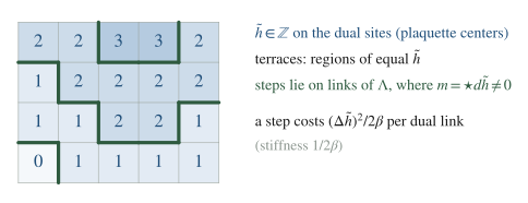
Figure 2. The height-model face of the XY model. Rough (wandering) surface ↔ low-$T$ QLRO phase of XY; smooth (frozen) surface ↔ high-$T$ disordered phase. Note the inversion: the surface temperature is $\propto 1/T_{\mathrm{XY}}$.

4. Third rewriting: spin waves and the Coulomb gas [Computed.]

One more Poisson resummation — on the heights — separates the smooth fluctuations from the integer charges.

Move 4 — Poisson on the heights. The heights of §3 are defined modulo a global integer shift, so $Z_{\mathrm{SOS}}^{(0)}$ is a sum over the quotient ${\mathbb{Z}}^{N^{\ast }}/\mathbb{Z}\cdot 1$, where $N^{\ast }$ is the number of dual sites and $1=(1,\dots ,1)$ is the constant cochain. Its Poisson dual integrates a real field $\tilde{\phi }$ over the cylinder ${\mathbb{R}}^{N^{\ast }}/\mathbb{Z}\cdot 1$, with the Lebesgue measure on one fundamental domain, against dual integers $v\in C^0({\Lambda }^{\ast },\mathbb{Z})$, one per dual site:

$$Z_{\mathrm{SOS}}^{(0)}=\sum _{v\in C^0({\Lambda }^{\ast },\mathbb{Z})}{\int }_{{\mathbb{R}}^{N^{\ast }}/\mathbb{Z}\cdot 1}\mathcal{D}\tilde{\phi }\exp (-\frac{1}{2\beta }\Vert d\tilde{\phi }{\Vert }^2+2\pi i\sum _{\tilde{x}}{v}_{\tilde{x}}{\tilde{\phi }}_{\tilde{x}}).$$

To derive it, we write the quotient sum as ${\sum }_{\tilde{h}\in {\mathbb{Z}}^{N^{\ast }}}F(\tilde{h})\rho (⟨\tilde{h},1⟩/N^{\ast })$, where $F$ is the Boltzmann weight and ρ is any function with ${\sum }_{k\in \mathbb{Z}}\rho (t+k)=1$, apply the Poisson identity of conventions §3 at every dual site, and fold the integral along $1$ back into one period, which is allowed because $F(\tilde{\phi })e^{2\pi iv\cdot \tilde{\phi }}$ is invariant under $\tilde{\phi }\to \tilde{\phi }+1$ for integer $v$. The quotient lattice still has covolume 1, so its dual lattice is still all of ${\mathbb{Z}}^{N^{\ast }}$ and no factor appears at this step. The real field $\tilde{\phi }$ is the spin-wave sector (a free Gaussian field, dual-lattice avatar of the §1 fluctuations); the integers $v_{\tilde{x}}$ (one per dual site, i.e. one per plaquette of Λ) are about to become the vortices. That they sit exactly where Week 1 §4.1 localized vortex charge is the first sign; §5 completes the identification.

Move 5 — the zero mode enforces neutrality. Write $\tilde{\phi }={\tilde{\phi }}_{0}1+{\tilde{\phi }}^{\prime }$ with ${\tilde{\phi }}^{\prime }\perp 1$ and ${\tilde{\phi }}_0\in [0,1)$, one period of the cylinder. The unit vector along $1$ is $1/\sqrt{N^{\ast }}$, so the coordinate along it is $\sqrt{N^{\ast }}{\tilde{\phi }}_0$ and the measure is $\mathcal{D}\tilde{\phi }=\sqrt{N^{\ast }}d{\tilde{\phi }}_0\mathcal{D}{\tilde{\phi }}^{\prime }$. The action does not contain ${\tilde{\phi }}_0$ ($d1=0$), but the source term does:

$$\sqrt{N^{\ast }}{\int }_0^{1}d{\tilde{\phi }}_0{e}^{2\pi i{\tilde{\phi }}_0{\sum }_{\tilde{x}}{v}_{\tilde{x}}}=\sqrt{N^{\ast }}{\delta }_{{\sum }_{\tilde{x}}{v}_{\tilde{x}},0}⟹\boxed{{\sum }_{\tilde{x}}{v}_{\tilde{x}}=0\text{ exactly,}}$$

a Kronecker delta, because $\sum v$ is an integer. Charge neutrality of the vortex gas is therefore a kinematic identity, enforced configuration by configuration by the compact zero mode, and it comes with the Jacobian $\sqrt{N^{\ast }}$, which we carry into $Z_{\mathrm{sw}}$ below. (On the infinite plane the same statement appears as “a charged configuration costs infinite energy”; the torus derivation is cleaner. Fine print F4.)

Move 6 — integrate the spin waves. What remains is a Gaussian integral over ${\tilde{\phi }}^{\prime }\perp 1$ with the imaginary source $J=2\pi v$. Complete the square explicitly: with Δ the Laplacian of ${\Lambda }^{\ast }$ (conventions §2, $\Delta \ge 0$), the action is $\frac{1}{2\beta }⟨{\tilde{\phi }}^{\prime },\Delta {\tilde{\phi }}^{\prime }⟩-i⟨J,{\tilde{\phi }}^{\prime }⟩$, and shifting ${\tilde{\phi }}^{\prime }={\tilde{\phi }}^{\prime \prime }+i\beta G^{\prime }J$ (legitimate contour rotation for a convergent Gaussian) gives

$$\frac{1}{2\beta }⟨{\tilde{\phi }}^{\prime \prime },\Delta {\tilde{\phi }}^{\prime \prime }⟩+\frac{\beta }{2}⟨J,G^{\prime }J⟩,$$

where $G^{\prime }={\Delta }^{-1}$ on the complement of the constants (Week 2 §6: the inverse exists exactly there), which is where $J$ lives after Move 5. So the ${\tilde{\phi }}^{\prime \prime }$ integral factors off as the free determinant and the sources are left with $e^{-\frac{\beta }{2}⟨J,G^{\prime }J⟩}$. With $J=2\pi v$, the exponent is $-\frac{\beta }{2}(2\pi {)}^2⟨v,G^{\prime }v⟩=-2{\pi }^2\beta ⟨v,G^{\prime }v⟩$. Assembling,

$$Z_{\mathrm{SOS}}^{(0)}=Z_{\mathrm{sw}}\cdot \sum _{\begin{array}{c}v\in C^0({\Lambda }^{\ast },\mathbb{Z})\\ \sum v=0\end{array}}\exp (-2{\pi }^2\beta \sum _{\tilde{x},\tilde{y}}{v}_{\tilde{x}}{G}^{\prime }(\tilde{x}-\tilde{y})v_{\tilde{y}}),$$

where

$$Z_{\mathrm{sw}}=\sqrt{N^{\ast }}{\int }_{{\tilde{\phi }}^{\prime }\perp 1}\mathcal{D}{\tilde{\phi }}^{\prime }{e}^{-\Vert d{\tilde{\phi }}^{\prime }{\Vert }^2/2\beta }=\sqrt{N^{\ast }}(2\pi \beta {)}^{(N^{\ast }-1)/2}(\det {}^{\prime }\Delta {)}^{-1/2}$$

is the free spin-wave partition function, Jacobian of Move 5 included, with $\det {}^{\prime }\Delta$ the product of the nonzero eigenvalues of Δ on ${\Lambda }^{\ast }$ (its correlators reproduce Week 1 §3; see §7). The factorization

$$\boxed{Z^{(0)}=(2\pi \beta {)}^{-N_{\ell }/2}{Z}_{\mathrm{sw}}{Z}_{\mathrm{Coulomb}}}$$

is exact within the zero-tilt sector: it is derived, term by term, from the Villain partition function with every prefactor displayed. The full $Z={\sum }_w{Z}^{(w)}$ multiplies this by the tilt theta function of §3, whose Gaussian value was computed there and whose vortex corrections do not affect bulk observables.

Move 7 — expose the Coulomb law and the fugacity. Insert $G^{\prime }(r)=G^{\prime }(0)-a(r)$, with $a(r)$ the exact subtracted Green function of Week 1 §3.3 ($a(0)=0$). On the $L\times L$ torus the same subtraction, $a=G^{\prime }(0)-G^{\prime }$, defines the torus function, which tends to the infinite-lattice $a$ of Week 1 as $L\to \infty$ at fixed separation. Using neutrality:

$$\sum _{\tilde{x},\tilde{y}}{v}_{\tilde{x}}{v}_{\tilde{y}}{G}^{\prime }(\tilde{x}-\tilde{y})=G^{\prime }(0)\underset{=0}{\underbrace{(\sum v{)}^2}}-\sum _{\tilde{x}\ne \tilde{y}}{v}_{\tilde{x}}{v}_{\tilde{y}}a(\tilde{x}-\tilde{y})$$

(diagonal terms of the second sum vanish since $a(0)=0$). The exact vortex weight is therefore

$$\boxed{Z_{\mathrm{Coulomb}}=\sum _{\begin{array}{c}v:\sum v=0\end{array}}\exp (2{\pi }^2\beta \sum _{\tilde{x}\ne \tilde{y}}{v}_{\tilde{x}}{v}_{\tilde{y}}a(\tilde{x}-\tilde{y})),}$$

with the exact lattice $a(r)$ at every separation — this much is an identity.

The long-distance normal form. To read off the physics, insert the asymptotics $a(r)=\frac{1}{2\pi }\ln r+\kappa +O(r^{-2})$ — exact only at large separation. With ${\sum }_{\tilde{x}\ne \tilde{y}}{v}_{\tilde{x}}{v}_{\tilde{y}}=(\sum v{)}^2-\sum v^2=-\sum v^2$ (neutrality), the constant κ reorganizes into a per-charge cost:

$$S_{\mathrm{Coulomb}}[v]\simeq -\pi \beta \sum _{\tilde{x}\ne \tilde{y}}{v}_{\tilde{x}}{v}_{\tilde{y}}\ln |\tilde{x}-\tilde{y}|+\underset{E_{\mathrm{core}}}{\underbrace{2{\pi }^2\beta \kappa }}\sum _{\tilde{x}}{v}_{\tilde{x}}^2,y\equiv e^{-E_{\mathrm{core}}}=e^{-2{\pi }^2\beta \kappa },\kappa =\frac{2{\gamma }_E+\ln 8}{4\pi }.$$

Read the status of each symbol correctly: the logarithmic interaction between well-separated charges is exact (the $O(r^{-2})$ tail is an irrelevant short-range correction); the fugacity $y$ is a long-distance matching convention, the value that reproduces the exact gas when all charges are far apart. Configurations with nearby charges see the exact $a(r)$, whose deviation from the asymptote is a finite set of short-range couplings that further renormalize $y$ (and generate the multi-charge fugacities of F6) without touching the log. In RG terms: $y=e^{-2{\pi }^2\beta \kappa }$ is the correctly normalized initial condition at the lattice scale, to leading order in the short-distance corrections — not an exact microscopic identity. This distinction matters when quoting numbers (Week 4, F2).

Check against Week 1. One $+$ at ${\tilde{x}}_1$, one $-$ at ${\tilde{x}}_2$, well separated: the double sum over ordered pairs gives $2\cdot (+1)(-1)\ln r_{12}$, so $S=2\pi \beta \ln r_{12}+2E_{\mathrm{core}}$ — exactly the pair energy $2\pi \beta \ln (r/a_0)+2E_{\mathrm{core}}$ estimated in Week 1 §4.3, with the core energy now identified in the long-distance normalization: $E_{\mathrm{core}}=2{\pi }^2\beta \kappa$, the lattice Green-function constant doing physics. Like charges repel, opposite charges attract logarithmically, the gas is neutral: the two-dimensional Coulomb gas, derived.

Physical picture. The Villain XY model is two decoupled theories wearing one set of variables: a free field that is critical at every temperature and never does anything dramatic (spin waves), and a neutral logarithmic plasma that undergoes a dielectric-to-conductor transition (vortices). The duality is valuable because it diagonalizes the Villain model into these sectors exactly in the zero-tilt sector of §3; with the winding sectors restored the spin waves still factor off exactly, and the vortices see the windings only through their total dipole moment, $\Theta (v)$ of §5 (F1). It is a statement about the Villain weight that the cosine model inherits only through the Villain approximation. The plasma’s fugacity comes with it, $y=e^{-2{\pi }^2\beta \kappa }$, in the long-distance matching convention of §4, where the constant κ of the asymptote of the lattice Green function, the one that normalized Week 1’s correlator, becomes a core energy by neutrality, and the short-distance deviations of $a(r)$ are left to renormalize $y$ further. When Week 4 tunes the vortex fugacity in the RG, this is the value it starts from, in that convention.

5. Cross-check: the lattice vorticity carries the same Coulomb gas [Proved.]

The integers $v$ of Move 4 come from a Poisson resummation of the heights, while the vorticity $dn$ of §1.2 is built from the Villain integers. They are different summation variables, and no continuum argument can identify them. What we prove instead is that the lattice vorticity $dn$ itself, with no dual variables at all, carries exactly the Coulomb gas of §4. The proof is two lines of Week 2 Hodge theory.

The Hodge split of the Villain action. Decompose the real 1-cochain $2\pi n$ into exact, co-exact and harmonic parts (Week 2 §6),

$$2\pi n=d\varphi +\delta \xi +h,\varphi \in C^0(\Lambda ,\mathbb{R}),\xi \in C^2(\Lambda ,\mathbb{R}),dh=\delta h=0.$$

Then $d\theta -2\pi n=d(\theta -\varphi )-\delta \xi -h$, and since the three pieces are mutually orthogonal,

$$\Vert d\theta -2\pi n{\Vert }^2=\Vert d(\theta -\varphi ){\Vert }^2+\Vert \delta \xi {\Vert }^2+\Vert h{\Vert }^2.$$

Applying $d$ to the decomposition removes $d\varphi$ and $h$, so $d\delta \xi =d(2\pi n)=2\pi dn=2\pi v$. In $d=2$ there are no 3-cells, so $\delta d=0$ on 2-cochains and $d\delta =\Delta$ there. The equation $\Delta \xi =2\pi v$ is solvable because ${\sum }_P{v}_P={\sum }_P(dn{)}_P=n({\sum }_P\partial P)=0$ on a closed surface (every link bounds two plaquettes, with opposite orientations), so $v$ is orthogonal to the constants, which are the kernel of Δ on 2-cochains. Therefore $\xi =2\pi G^{\prime }v$ up to a constant, which δ annihilates, and

$$\Vert \delta \xi {\Vert }^2=⟨\xi ,d\delta \xi ⟩=⟨2\pi G^{\prime }v,2\pi v⟩=4{\pi }^2⟨v,G^{\prime }v⟩,$$

where $G^{\prime }$ is the inverse of Δ on the 2-cochains orthogonal to the constants. Transported by ⋆, Δ on 2-cochains is the site Laplacian of ${\Lambda }^{\ast }$ (each plaquette couples to its four neighbours across its four links), so $G^{\prime }$ is the kernel $G^{\prime }(\tilde{x}-\tilde{y})$ of Move 6. The Villain weight of every configuration $(\theta ,n)$ thus splits as

$$e^{-\frac{\beta }{2}\Vert d\theta -2\pi n{\Vert }^2}=e^{-\frac{\beta }{2}\Vert d(\theta -\varphi ){\Vert }^2}{e}^{-2{\pi }^2\beta ⟨v,G^{\prime }v⟩}{e}^{-\frac{\beta }{2}\Vert h{\Vert }^2},v=dn,$$

where the middle factor is the Coulomb weight of §4, with the same coefficient $2{\pi }^2\beta$. Neutrality needs no zero-mode argument here, since ${\sum }_P(dn{)}_P=0$ identically.

The partition function. The branch redundancy of §1.2 lets θ range over the cylinder ${\mathbb{R}}^{N_s}/2\pi \mathbb{Z}\cdot 1$, with $N_s$ the number of sites, provided we keep one representative $n$ per class of $C^1(\Lambda ,\mathbb{Z})/d{C}^0(\Lambda ,\mathbb{Z})$. On the cylinder the shift $\theta \to \theta +\varphi$ removes φ, so the θ integral gives the same number for every class,

$$Z_{\mathrm{G}}={\int }_{{\mathbb{R}}^{N_s}/2\pi \mathbb{Z}\cdot 1}\prod _x\frac{d{\theta }_x}{2\pi }{e}^{-\frac{\beta }{2}\Vert d\theta {\Vert }^2}=\sqrt{N_s}(2\pi \beta {)}^{-(N_s-1)/2}(\det {}^{\prime }\Delta {)}^{-1/2},$$

where the $\sqrt{N_s}$ comes from the zero mode, as in Move 5, and $\det {}^{\prime }\Delta$ now refers to the sites of Λ. A class is fixed by $v=dn$, which can be any neutral integer 2-cochain, together with the two winding numbers $t\in {\mathbb{Z}}^2$ of $n$ (the integer cohomology of the torus has no torsion), and $h$ depends only on these. Therefore, exactly,

$$\boxed{Z=Z_{\mathrm{G}}\sum _{\begin{array}{c}v\in C^2(\Lambda ,\mathbb{Z})\\ \sum v=0\end{array}}{e}^{-2{\pi }^2\beta ⟨v,G^{\prime }v⟩}\Theta (v),\Theta (v)=\sum _{t\in {\mathbb{Z}}^2}{e}^{-\frac{\beta }{2}\Vert h(v,t){\Vert }^2},}$$

and $h$ carries the winding sectors. At $v=0$ the cochain $n$ is closed with windings $t$, so $h=\frac{2\pi }{L}(t_1{h}^{(1)}+t_2{h}^{(2)})$ with $h^{(i)}$ the harmonic cochains of Week 2 §6, and $\frac{\beta }{2}\Vert h{\Vert }^2=2{\pi }^2\beta |t{|}^2$. $\square$

The two routes compared. At $v=0$ the prefactors can be compared one by one. On the $L\times L$ torus $N_{\ell }=2N_s$ and $N^{\ast }=N_s$, and the dual route gives, at $v=0$ and summed over tilt sectors, $(2\pi \beta {)}^{-N_s}{Z}_{\mathrm{sw}}{\sum }_w{e}^{-|w{|}^2/2\beta }$, because the Gaussian tilt weights of §3 are exact when no vortex is present. The Poisson identity ${\sum }_w{e}^{-w^2/2\beta }=\sqrt{2\pi \beta }{\sum }_t{e}^{-2{\pi }^2\beta t^2}$, used in each direction, turns this into $\sqrt{N_s}(2\pi \beta {)}^{-N_s+\frac{N_s-1}{2}+1}(\det {}^{\prime }\Delta {)}^{-1/2}{\sum }_t{e}^{-2{\pi }^2\beta |t{|}^2}$, which is $Z_{\mathrm{G}}\Theta (0)$ (the dual torus is isomorphic to Λ, so the two determinants coincide). Note that the $\sqrt{N^{\ast }}$ of Move 5 is exactly what this comparison needs. For $v\ne 0$ the comparison also goes through configuration by configuration: $\Theta (v)$ depends on $v$ only through its dipole moment ${\sum }_P{v}_P{x}_P$ (defined modulo $L$), the dual route sees the same dipole moment through the vortex corrections to the tilt weights, and a Poisson resummation matches the two [Sketched: the omitted step is the Poisson resummation of the tilt sum weighted by the dipole phase, as in F3]. In this precise sense the integers of Move 4 are the vorticity: the two exact routes give every neutral configuration the same weight.

The continuum reading [Heuristic.]. In the continuum the same decoupling is usually argued by splitting

$$\theta =\psi +{\theta }_v,$$

where ${\theta }_v$ is a fixed representative carrying the vortex content ($\nabla {\theta }_v$ is divergence-free, with $\oint \nabla {\theta }_v\cdot d\ell =2\pi v$ around each core) and ψ is a smooth, single-valued fluctuation. The energy splits as

$$E[\theta ]=\frac{\beta }{2}\int |\nabla \psi {|}^2+\beta \int \nabla \psi \cdot \nabla {\theta }_v+\frac{\beta }{2}\int |\nabla {\theta }_v{|}^2,$$

and the cross term vanishes,

$$\int \nabla \psi \cdot \nabla {\theta }_v=-\int \psi {\nabla }^2{\theta }_v+{\oint }_{\partial }\psi \nabla {\theta }_v\cdot d\vec{S}=0,$$

because ${\nabla }^2{\theta }_v=0$ (the singular part of $\nabla {\theta }_v$ at the cores is its curl), ψ is single-valued, and the boundary term vanishes on the torus. This is the physical content of the lattice proof: $-\delta \xi$ is the lattice $\nabla {\theta }_v$ (co-closed, with $d(-\delta \xi )=-2\pi v$ as in §1.2), $d(\theta -\varphi )$ is the lattice $\nabla \psi$, and their orthogonality is the vanishing of the cross term. The decoupling of spin waves and vortices is the harmonicity of the vortex configuration, and the Hodge split is its exact lattice form, with no choice of representative and no continuum approximation.

6. Fourth face: sine-Gordon [Controlled to $O(y^2)$ in the fugacity, both directions.]

The Coulomb gas has a field-theory generating function, and its field is already on the page. Consider the real field $\chi =2\pi {\tilde{\phi }}^{\prime }$ on dual sites, with ${\tilde{\phi }}^{\prime }$ the real height of Moves 4–6. Its Gaussian action is $\frac{1}{2\beta }\Vert d{\tilde{\phi }}^{\prime }{\Vert }^2=\frac{1}{8{\pi }^2\beta }\Vert d\chi {\Vert }^2$, so its covariance is $⟨{\chi }_{\tilde{x}}{\chi }_{\tilde{y}}⟩=4{\pi }^2\beta G^{\prime }(\tilde{x}-\tilde{y})$, and the source term of Move 4 is $e^{2\pi iv\cdot {\tilde{\phi }}^{\prime }}=e^{iv\cdot \chi }$. Move 6 therefore reads, for any neutral charge configuration,

$$⟨e^{i{\sum }_{\tilde{x}}{v}_{\tilde{x}}{\chi }_{\tilde{x}}}{⟩}_{\chi }=\exp (-\frac{1}{2}4{\pi }^2\beta \sum v{G}^{\prime }v)=\exp (-2{\pi }^2\beta \sum v{G}^{\prime }v),$$

where $⟨\cdot {⟩}_{\chi }$ is the normalized Gaussian average: exactly the Coulomb weight. (If the zero mode of χ is integrated over one period, as in Move 5, a non-neutral configuration averages to zero, and the sum over charges may run over all of $C^0({\Lambda }^{\ast },\mathbb{Z})$.) Summed over all integers at every site, ${\sum }_{v\in \mathbb{Z}}{e}^{iv\chi }=2\pi {\sum }_{k\in \mathbb{Z}}\delta (\chi -2\pi k)$ pins $\chi /2\pi$ to the integers and the heights of §3 return; the cosine potential below is this Poisson comb, truncated.

The vertex normalization. Two steps are not identities. (a) We truncate to $|v_{\tilde{x}}|\le 1$ (justified in F6): ${\sum }_{v\in \{0,\pm 1\}}{e}^{iv\chi }=1+2\cos \chi$, so the truncated gas is exactly $⟨{\prod }_{\tilde{x}}(1+2\cos {\chi }_{\tilde{x}}){⟩}_{\chi }$. We state the normalization of the vertex once. With bare vertex operators and the exact kernel, the coupling is $2\cos \chi$ with unit coefficient, and the fugacity emerges from $a(r)$ through the self-contraction of the vertices,

$$⟨e^{i{\chi }_{\tilde{x}}}{e}^{-i{\chi }_{\tilde{y}}}{⟩}_{\chi }=e^{-\frac{1}{2}⟨({\chi }_{\tilde{x}}-{\chi }_{\tilde{y}}{)}^2⟩}=e^{-4{\pi }^2\beta a(\tilde{x}-\tilde{y})}=y^2|\tilde{x}-\tilde{y}{|}^{-2\pi \beta }[1+O(r^{-2})],y=e^{-2{\pi }^2\beta \kappa },$$

where we used $4{\pi }^2\beta a(r)=2\pi \beta \ln r+4{\pi }^2\beta \kappa +O(r^{-2})$; more generally, a neutral configuration of $n$ unit charges, all far apart, carries exactly $y^n$ (§4). With vertices normal-ordered at the lattice scale, $V_{\pm }(\tilde{x})\equiv y^{-1}{e}^{\pm i{\chi }_{\tilde{x}}}$, whose correlators have unit amplitude at long distance, the same identity reads $1+2\cos {\chi }_{\tilde{x}}=1+2yV(\tilde{x})$ with $V=\frac{1}{2}(V_{+}+V_{-})$: the coupling is $y$. This is the normalization of conventions §5, and from now on we use it and write $\cos \chi$ for $V$. The two schemes place the same number differently, and combining $y$ with bare vertices counts the core energy twice (F5). (b) We exponentiate, ${\prod }_{\tilde{x}}(1+2y\cos {\chi }_{\tilde{x}})\simeq \exp \left(2y{\sum }_{\tilde{x}}\cos {\chi }_{\tilde{x}}\right)$; the difference consists of terms with two or more vertices on one dual site, which the continuum theory excludes by its cutoff at $a_0$ (the hard core of the lattice gas) and which F6 shows to shift only nonuniversal constants. With ${\sum }_{\tilde{x}}\to \int d^{2}x$ ($a_0=1$),

$$\boxed{Z_{\mathrm{Coulomb}}\simeq \int \mathcal{D}\chi \exp (-\int d^{2}x[\frac{1}{8{\pi }^2\beta }(\partial \chi {)}^2-2y\cos \chi ]),}$$

which is sine-Gordon, with stiffness $1/(2\pi {)}^2\beta$ (continuum normalization $\frac{1}{8{\pi }^2\beta }$) and the vertex operator $e^{\pm i\chi }$ inserting a $\pm$ charge.

Physical picture. χ is the disorder field: its vertex operator creates a vortex, exactly as $e^{i\theta }$ creates a charge — the two fields are each other’s dark side, and neither is more fundamental. The $\cos \chi$ potential is the amplitude for the vacuum to nucleate vortex–antivortex pairs; when it is irrelevant the vacuum stays a dielectric of bound pairs, and when it is relevant the field χ gets pinned at a minimum — a “vortex condensate” — which is the disordered phase. Pinning χ gaps it, and with it every correlation of the dual theory: this “the disorder field acquires a gap-generating potential from proliferating defects” mechanism is precisely Polyakov’s confinement mechanism one dimension up (Week 8–Week 10), where χ becomes the dual photon and the defects become monopoles. Learn the mechanism here, where nothing else is going on.

The $O(y^2)$ match, both directions. From the Coulomb gas to sine-Gordon. By the identity above, each one-pair term of the gas, a $+$ at $\tilde{x}$ and a $-$ at $\tilde{y}$, is the two-vertex term $⟨e^{i{\chi }_{\tilde{x}}}{e}^{-i{\chi }_{\tilde{y}}}{⟩}_{\chi }=e^{-4{\pi }^2\beta a(\tilde{x}-\tilde{y})}$ of $⟨\prod (1+2\cos \chi ){⟩}_{\chi }$, exactly; at long distance it equals $y^2{r}^{-2\pi \beta }$, the one-pair Boltzmann weight $e^{-2\pi \beta \ln r-2E_{\mathrm{core}}}$ of §4. From sine-Gordon to the Coulomb gas. We expand the boxed weight to second order in $y$ and contract with the Gaussian χ, with normal-ordered vertices. The $O(y)$ term vanishes by neutrality (the zero mode of χ). At $O(y^2)$ the same-sign products $⟨V_{\pm }{V}_{\pm }⟩$ vanish for the same reason, and

$$\frac{(2y{)}^2}{2}\int \int d^{2}x{d}^2{x}^{\prime }⟨\cos \chi (x)\cos \chi (x^{\prime })⟩=\frac{y^2}{2}\int \int d^{2}x{d}^2{x}^{\prime }[⟨V_{+}(x)V_{-}(x^{\prime })⟩+⟨V_{-}(x)V_{+}(x^{\prime })⟩]=y^2\int {\int }_{|x-x^{\prime }|>1}{d}^{2}x{d}^2{x}^{\prime }|x-x^{\prime }{|}^{-2\pi \beta },$$

where the cutoff excludes coincident vertices. This is the one-pair sector of the Coulomb gas in its long-distance normal form, one term for each placement of the $+$ and the $-$, with the same $y^2$ and the same power. $\square$

The number Week 4 needs. From the same contraction,

$$⟨e^{i\chi (\tilde{x})}{e}^{-i\chi (0)}⟩\sim |\tilde{x}{|}^{-2\pi \beta }⟹{\Delta }_{\mathrm{vortex}}=\pi \beta .$$

The vortex insertion is a scaling operator of dimension $\pi \beta$: relevant when $\pi \beta <2$ ($y$ grows: plasma), irrelevant when $\pi \beta >2$ (bound dipoles), marginal at $\beta =2/\pi$ — precisely Week 1’s energy–entropy threshold, now derived as an operator dimension. Week 4 turns this into the Kosterlitz flow.

6.1 The operator content of the fixed line [Computed.]

Collect the dimensions of all the exponential operators on the Gaussian fixed line of stiffness ${\beta }_R$ — both the order (electric) operators $e^{iq\theta }$ of Week 1 and the disorder (magnetic) operators $e^{ip\chi }$ of this week:

$${\Delta }_q^{\mathrm{el}}=\frac{q^2}{4\pi {\beta }_R}(\text{from }⟨e^{iq\theta }{e}^{-iq\theta }⟩\sim r^{-q^2/2\pi {\beta }_R}),{\Delta }_p^{\mathrm{mag}}=\pi {\beta }_R{p}^2(\text{from above}).$$

operator	dimension	relevant when	role
$e^{i\theta }$ (spin)	$1/4\pi {\beta }_R$	always ($\Delta <2$ in QLRO)	order probe; $\eta =2{\Delta }_1^{\mathrm{el}}$
$e^{iq\theta }$	$q^2/4\pi {\beta }_R$	small $q$	higher-charge probes
$e^{i\chi }$ (vortex)	$\pi {\beta }_R$	$\pi {\beta }_R<2$	drives BKT
$e^{ip\chi }$	$\pi {\beta }_R{p}^2$	far in the plasma phase only	multi-vortex (Week 3 F6: negligible)

Two structural facts sit in this table. First, the β-independent product

$${\Delta }_q^{\mathrm{el}}\cdot {\Delta }_p^{\mathrm{mag}}=\frac{q^2{p}^2}{4},$$

the fingerprint of the underlying free-boson ("$c=1$") critical line: electric and magnetic dimensions see the coupling reciprocally, and their product is pure integer data. Second, integer charges $q$ and vortices $p$ are mutually local (monodromy phase $e^{2\pi iqp}=1$), but fractional values would braid nontrivially — the germ of anyonic statistics, realized for real in the toric code (Semester II Week 8), where exactly such mutual monodromies between “electric” and “magnetic” excitations become the physical observable. The XY fixed line is the simplest place where the electric/magnetic operator pairing — the engine of Semester II — can be seen whole.

7. Charge correlators through the duality [Computed in the spin-wave sector; dressing Sketched.]

What of the original observable $⟨e^{i{\theta }_x}{e}^{-i{\theta }_y}⟩$? Repeat Moves 1–3 with the insertions. The extra factor $e^{i({\theta }_x-{\theta }_y)}$ shifts the Kronecker constraint at the two marked sites:

$$\int \frac{d{\theta }_z}{2\pi }{e}^{i[(\delta m{)}_z+{ϵ}_z]{\theta }_z}={\delta }_{(\delta m{)}_z,-{ϵ}_z},ϵ=1_x-1_y,$$

so $\delta m=-ϵ$ and the dual current is no longer conserved. Since $\delta m$ is inflow minus outflow (conventions §2), $(\delta m{)}_x=-1$ makes $x$ a unit source and $(\delta m{)}_y=+1$ makes $y$ a unit sink: every configuration contains an open current line from $x$ to $y$ (plus closed loops). The charge correlator is a sum over integer flux lines connecting the insertions, the lattice ancestor of “a charged operator trails a Wilson line.”

To evaluate, split off one fixed unit current $m_{\gamma }$ along a chosen path ${\gamma }_{x\to y}$ (so $\delta m_{\gamma }=-ϵ$) and write $m=m_{\gamma }+m^{\prime }$ with $\delta m^{\prime }=0$ integer. The weight splits as

$$\Vert m{\Vert }^2=\Vert m_{\gamma }{\Vert }^2+2m_{\gamma }\cdot m^{\prime }+\Vert m^{\prime }{\Vert }^2.$$

Run Moves 4–6 on $m^{\prime }$: heights, then Poisson, then the Gaussian field $\tilde{\phi }$ with vortex charges $v$. In the Gaussian ($v=0$) sector, the cross term contributes a real linear source for $\tilde{\phi }$, and the whole computation reduces to one orthogonality argument [Computed]:

Step 1 — decompose the fixed current. We work on the infinite lattice, where a current of finite support has no harmonic part, and Hodge-decompose $m_{\gamma }$ over the reals (Week 2 §6):

$$m_{\gamma }=dg+\star d\lambda ,\delta m_{\gamma }=\delta dg=\Delta g=-ϵ⟹g=-G\ast ϵ,$$

where the co-closed piece $\star d\lambda$ carries no divergence and $g$ is the lattice Coulomb potential of the endpoint charges. (On the $L\times L$ torus $m_{\gamma }$ also has a harmonic part, of norm ${\sum }_i{\Delta }_i^2/L^2$ for a path of net displacement $\Delta$; it combines with the tilt sectors of §3 into a factor that tends to 1 as $L\to \infty$ at fixed $x-y$. Problem 1(b) meets it on the $2\times 2$ torus.)

Step 2 — the sum over $m^{\prime }$ absorbs the co-closed piece. The fluctuation integral over the dual field is a shifted Gaussian; shifting $\tilde{\phi }$ by the fixed function $\lambda$ (allowed: $\tilde{\phi }$ ranges over all reals) cancels the cross term $m_{\gamma }\cdot m^{\prime }$ against the co-closed part of $m_{\gamma }$ exactly — the Gaussian sector cannot tell a co-closed background from its own fluctuations. What survives of $\Vert m_{\gamma }{\Vert }^2+2m_{\gamma }\cdot m^{\prime }$ after the shift is only the exact piece:

$$\text{surviving exponent}=-\frac{1}{2\beta }\Vert dg{\Vert }^2.$$

Step 3 — evaluate the exact piece. By adjointness and Step 1,

$$\Vert dg{\Vert }^2=⟨g,\delta dg⟩=⟨g,-ϵ⟩=⟨G\ast ϵ,ϵ⟩=2[G(0)-G(x-y)]=2a(x-y),$$

using $ϵ=1_x-1_y$ in the last line. Therefore

$$⟨e^{i{\theta }_x}{e}^{-i{\theta }_y}{⟩}_{\mathrm{sw}}=\exp [-\frac{1}{\beta }a(x-y)],$$

exactly — path-independence is now manifest (the answer depends on $m_{\gamma }$ only through $\delta m_{\gamma }=-ϵ$: any two choices of path differ by a conserved current, which Step 2 absorbs; on the torus a difference that winds is absorbed instead by relabeling the tilt sectors, Problem 1(b)). Expanding $a$ at large distance, this is $e^{-\kappa /\beta }|x-y{|}^{-1/2\pi \beta }$: Week 1’s spin-wave answer — exponent and amplitude, and in fact the full exact lattice function $e^{-a(x-y)/\beta }$, not merely its asymptote — recovered from the dual side. No factor was dropped anywhere in Moves 1–6 (the Jacobian $\sqrt{N^{\ast }}$ of Move 5 included), and all of them are common to the numerator and to $Z$; this is the strongest available consistency check on the whole chain. The vortex charges couple to the open line through the angle it subtends; at low temperature (bound dipoles) they renormalize the amplitude $e^{-\kappa /\beta }$ and $\beta \to {\beta }_R$ but preserve the power law; in the plasma phase they screen the line into exponential decay [Sketched — the full dressing is JKKN §III; Problem 3 develops the leading correction]. This is the mechanism by which the same transition shows up in the original spin variables.

8. The duality dictionary

Figure 3 collects the faces of the model and the exact routes between them, the direct route of §5 included, and the table below translates each object across the four columns.

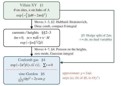
Figure 3. The faces of the Villain XY model and the exact routes between them: Moves 1–7 through currents and heights, and the direct Hodge route of §5; only the step to sine-Gordon is approximate.

XY / spin language	current model	height (SOS) model	Coulomb gas / sine-Gordon
phase ${\theta }_x$ (compact, sites of Λ)	integer current $m$ on links, $\delta m=0$ (Moves 1–3)	integer height $\tilde{h}$ on dual sites; real height $\tilde{\phi }$ after Move 4	dual field $\chi =2\pi \tilde{\phi }$ (dual sites)
stiffness β	loop weight $e^{-m^2/2\beta }$	surface stiffness $1/2\beta$	plasma coupling $\pi \beta$; SG stiffness $\frac{1}{(2\pi {)}^2\beta }$
charge operator $e^{i\theta }$	endpoint of an open current line: source at $e^{i\theta }$, sink at $e^{-i\theta }$ (§7)	screw dislocation of $\tilde{h}$: since $\delta m\ne 0$ at the insertion, $\tilde{h}$ gains $(\delta m{)}_x=-1$ once counter-clockwise around it	χ winds by $2\pi$ around the insertion; dimension $1/4\pi \beta$
vortex $v=dn$ (plaquettes)	— (it enters only through the integrality of $m$)	pinning vertex $e^{2\pi i\tilde{\phi }}$, the roughening potential	Coulomb charge; vertex $e^{\pm i\chi }$, coupling $2y\cos \chi$
ordered tendency (large β)	dense loops	rough surface	bound dipoles; $\cos \chi$ irrelevant
disordered (small β)	dilute loops	smooth surface	free plasma; $\cos \chi$ relevant
lattice constant κ (Week 1)	—	—	fugacity $y=e^{-2{\pi }^2\beta \kappa }$

The four faces describe one partition function, and every equality between them is exact except the two dilute-gas steps (a) and (b) of §6. Two pairings in the table are easy to invert. The charge operator $e^{i\theta }$ makes the currents end, so the height is multivalued around it (a screw dislocation) and χ winds around it. The vortex is the Poisson conjugate of the height, the pinning vertex $e^{2\pi i\tilde{\phi }}$ whose relevance decides between the smooth and the rough surface; the phase of bound dipoles, where the pinning is irrelevant, is therefore the rough one, as in §3 and Figure 2. This is the first full column-set of the semester’s duality table; Week 8 adds the gauge rows, and Semester II Week 12 upgrades the whole table to exact operator statements.

9. Subtleties and fine print

F1 — What “exact factorization” rests on. $Z^{(0)}=(\cdots )Z_{\mathrm{sw}}{Z}_{\mathrm{Coulomb}}$ came from two structural facts: the exact solvability of the constraint $\delta m=0$ by heights within a tilt sector (§3) and the linearity of the source coupling $2\pi iv\cdot \tilde{\phi }$ (so the Gaussian integral factorizes, §4). The tilt sectors themselves do not factor off exactly (§3): only their Gaussian weights are cleanly computable, which suffices for bulk physics. Perturb the model non-Gaussianly (e.g. cosine instead of Villain) and factorization becomes approximate: the vortex core acquires a size and spin-wave–vortex interactions appear at short distance. They renormalize $y$ and β but generate no new relevant couplings — which is why the universal content survives (F2).

F2 — Villain vs cosine = a fugacity shift. Matching the two models’ character expansions (Week 1, Problem 5) fixes $\tilde{\beta }(\beta )$ by the first harmonic; the residual mismatch in the higher harmonics is then algebraically small in $1/\beta$ (the $m=2$ coefficient first disagrees at subleading order in the $1/\beta$ expansions of $e^{-m^2/2\tilde{\beta }}$ vs $I_m/I_0$ — power-law, not exponentially, suppressed). In Coulomb-gas language: a shifted core energy and small multi-charge fugacities. Consequently the numerical value of $T_{BKT}$ differs between the models, and neither equals the naive $2/\pi$: the Monte Carlo bare critical couplings are ${\beta }_c^{\cos }\approx 1.12$ and ${\beta }_c^{\mathrm{Vil}}\approx 0.75$ [Stated — refs: Hasenbusch, J. Phys. A 38 (2005) 5869, for the cosine model; Janke and Nather, Phys. Rev. B 48 (1993) 7419, for the Villain model], both well above $2/\pi \approx 0.64$ because screening lowers the renormalized stiffness (Week 4). The transition’s existence, the flow, the jump, and all exponents coincide (universal). When comparing with data, match renormalized stiffnesses, never bare couplings.

F3 — The tilt (winding) sectors. The sector weights $Z^{(w)}/Z^{(0)}\simeq e^{-(w_1^2+w_2^2)/2\beta }$ (Gaussian level, §3) carry the global-current and twisted-boundary-condition physics. A twist α across the $x$-cycle adds α to the Villain field strength $(d\theta -2\pi n{)}_{\ell }$ on the seam, the column of $x$-links crossed by one vertical dual cycle. In Move 1 this multiplies the integrand by $e^{i\alpha {\sum }_{\ell \in \mathrm{seam}}{b}_{\ell }}$, and Move 2 sets $b=m$, so the twist enters as the phase $e^{i\alpha \cdot (\text{current through the seam})}$ on each configuration. That current is $w_1$ for every divergence-free $m$, since $\star d\tilde{h}$ has no net flux through a closed dual cycle; therefore, exactly and then at the Gaussian level,

$$Z(\alpha )=\sum _{w_1,w_2}{e}^{i\alpha w_1}{Z}^{(w)},\frac{Z(\alpha )}{Z(0)}\simeq \frac{{\sum }_w{e}^{-w^2/2\beta +i\alpha w}}{{\sum }_w{e}^{-w^2/2\beta }}=\frac{{\sum }_k{e}^{-\beta (\alpha -2\pi k{)}^2/2}}{{\sum }_k{e}^{-2{\pi }^2\beta k^2}},$$

where the last step is the Poisson identity of conventions §3, which trades the tilt $w$ for the θ-winding number $k$; only in this variable does α appear as a shift. Differentiating twice at $\alpha =0$ gives the exact winding-number estimator ${\rm Y}=⟨w_1^2⟩$ (the one worm algorithms use), and at the Gaussian level ${\rm Y}=\beta -{\beta }^2⟨(2\pi k{)}^2⟩=\beta [1+O(\beta e^{-2{\pi }^2\beta })]$, with $⟨\cdot ⟩$ weighted by $e^{-2{\pi }^2\beta k^2}$: the spin-wave stiffness of Week 1 Problem 6. A shift $w_1\to w_1+\alpha /2\pi$ inside the tilt theta function would instead give ${\rm Y}=⟨k^2⟩\simeq 2e^{-2{\pi }^2\beta }$, about $5\times 10^{-9}$ at $\beta =1$, which is the stiffness of the dual model at coupling $1/4{\pi }^2\beta$. Note that the weights are $L$-independent at fixed β: the unit-winding configuration relaxes to tilt density $1/L$ on each of the $L^2$ links of one orientation, and $L^2\times (1/L{)}^2=1$, so global tilts are not suppressed by the volume. They are invisible in bulk correlators at any fixed separation and decisive for stiffness measurements, so dropping the tilt sum is legitimate only after deciding which observable one wants.

F4 — Neutrality: finite vs infinite volume. On the torus, neutrality came from the zero-mode integral of Move 5, over one period of the cylinder: an identity, with no energetics in it. The period matters. The global integer shift of the heights is a redundancy, divided out once, so ${\tilde{\phi }}_0$ runs over $[0,1)$ and produces a Kronecker delta together with the Jacobian $\sqrt{N^{\ast }}$; integrating ${\tilde{\phi }}_0$ over all of $\mathbb{R}$, as if every height ranged over $\mathbb{Z}$ independently, would produce $\delta (\sum v)$, a Dirac delta evaluated on an integer. In the Hodge route of §5 neutrality is automatic, ${\sum }_P(dn{)}_P=0$. On the infinite plane one instead says “a net charge costs $\sim \ln L\to \infty$.” The two statements match: the zero mode is the $k\to 0$ limit that makes $G(x)$ itself ill-defined in 2d (Week 1, F5). Systems with a neutralizing background (e.g. an applied “magnetic field” term in JKKN) evade the constraint by modifying exactly this mode.

F5 — One self-energy, three appearances. The constant κ enters as (i) the amplitude of Week 1’s spin-wave correlator, (ii) the vortex core energy $E_{\mathrm{core}}=2{\pi }^2\beta \kappa$, (iii) the lattice-scale part of the self-contraction of the bare vertex $e^{i\chi }$, which normal ordering at the lattice scale moves into the coupling $y$ (§6). These are the same number seen through three calculations; any consistent scheme keeps it in exactly one place. Double-counting κ (a classic error) shifts the fugacity by a spurious square.

F6 — The two dilute-gas steps, and why they are safe. §6 (a) truncated to $|v|\le 1$ and (b) exponentiated $1+2y\cos \chi$. Both are controlled by operator dimensions: the charge-2 vertex has dimension $4\pi \beta =4\times$(charge-1) — strongly irrelevant near the transition ($\pi \beta \approx 2$ ⟹ dimension ≈ 8 vs marginality at 2); and the difference $e^{2y\cos \chi }-(1+2y\cos \chi )$ starts at $O(y^2)$ with the same operators already present. Neither step touches universal content; both shift non-universal constants only.

10. Common misconceptions

• “The Villain model is an uncontrolled approximation to the real XY model.” The Villain model is a well-defined lattice model in the same universality class, with its own exact duality — that is why we compute in it. The relation to the cosine model is a quantified, irrelevant deformation (F2), not an unexamined replacement.
• “Spin waves drive the transition.” The spin-wave sector is critical at every temperature and completely transition-blind; all non-analyticity lives in the Coulomb factor. What spin waves do is fix the vortex interaction (the log) and the critical correlators — the stage, not the play.
• “Duality maps the XY model to a different theory.” Every arrow in §§2–4 is an identity of partition functions: currents, heights, and the Coulomb gas are the same theory in different variables. “Dual” means a change of basis that makes different physics manifest, not a new model. (Semester II sharpens this: dualities are operators inside the theory.)
• “Vortices are inserted by hand into the Gaussian theory.” They were never absent: the integers $n_{\ell }$ are part of the compact model’s definition, and $v=dn$ emerged from resummation, uninvited. It is the Gaussian model of Week 1 §3 that was obtained by hand-deletion.

11. Historical note

Villain (1975) introduced the periodic Gaussian precisely to make the low-temperature expansion of the XY model tractable; José, Kadanoff, Kirkpatrick and Nelson (1977) turned it into the systematic spin-wave/vortex decomposition reproduced here, extended it to ${\mathbb{Z}}_N$ clock models and symmetry-breaking fields, and connected the fugacity expansion to Kosterlitz’s RG. The height-model face goes back to the same era’s crystal-surface literature (Chui–Weeks: roughening = inverted BKT). Fröhlich and Spencer (1981) made the whole picture rigorous — their proof that the Coulomb gas has a dipole phase at large β is, mathematically, the existence proof of the BKT transition, built on the identical representation derived in §4.

12. What to take away

1. The duality is four exact rewritings: Villain → conserved currents (compactness ⟹ integer Kronecker constraints) → heights + windings (integer Hodge) → spin waves + neutral Coulomb gas (Poisson + zero mode). Every constant tracked; factorization exact in the zero-tilt sector (F1).
2. The vortex gas comes out quantitative: interaction $-\pi \beta {\sum }_{\ne }vv\ln r$, exact neutrality from the zero mode, and fugacity $y=e^{-2{\pi }^2\beta \kappa }$ with κ the Week-1 lattice constant, in the long-distance matching convention of §4 — the value the RG of Week 4 starts from.
3. Sine-Gordon is the same theory once more, with the vortex operator $e^{i\chi }$ of dimension $\pi \beta$: relevant/irrelevant across $\beta =2/\pi$. That single dimension is Week 4’s input.
4. The mechanism of decoupling is orthogonality (§5): in the Hodge split of $2\pi n$ the vortex part of the Villain field strength is co-exact and the spin-wave part exact, so they cannot exchange energy at quadratic order; in the continuum this is the harmonicity of the vortex configuration, and it is the physical reason a free field and a plasma coexist in one model without mixing.

13. Looking ahead: Week 4

We hold an exact Coulomb gas with a computed fugacity and a vortex operator of dimension $\pi \beta$. Week 4 asks when the dipoles ionize: the energy–entropy argument, then Kosterlitz’s renormalization group — $dy/d\ell =(2-\pi {\beta }_R)y$ and the screening-driven flow of ${\beta }_R$ — the universal stiffness jump ${\rho }_s/T_{BKT}=2/\pi$, and the essential singularity of the correlation length. Then the week pivots to the Ising model’s Kramers–Wannier duality and the Kadanoff–Ceva disorder operator: the ℤ₂ sibling of everything done here, and the first duality implemented by a defect — the seed of Semester II’s non-invertible symmetries.

14. Problem set

Problems 1–3 are the classroom core, solvable from §§2–7; Problems 4⋆, 5⋆ and 7⋆ are self-study consolidation, each with a hint; Problem 6⋆⋆ is a research extension and states what is known, what is explored and what counts as completion.

Core problems (everyone).

1. The correlator through the duality, extended. (a) Repeat §7’s three steps for charge-$q$ insertions ($ϵ\to qϵ$) and show $⟨e^{iq{\theta }_x}{e}^{-iq{\theta }_y}{⟩}_{\mathrm{sw}}=e^{-q^{2}a(x-y)/\beta }$, recovering the $q^2\eta$ of Week 1 Problem 3 with the exact amplitude. (b) On the $2\times 2$ torus, take $x=(0,0)$ and $y=(1,0)$, and two paths from $x$ to $y$ that differ by the boundary of one plaquette: the single link ${\ell }_1(0,0)$, and the three-link path around the plaquette $P(0,0)$, up ${\ell }_2(0,0)$, along ${\ell }_1(0,1)$ and down ${\ell }_2(1,0)$. For both, split $m_{\gamma }$ into its exact, co-exact and harmonic parts, compute $\Vert m_{\gamma }{\Vert }^2$, $\Vert dg{\Vert }^2$ and the harmonic norm, and check that the two co-exact parts differ by the boundary current of one plaquette, which Step 2’s shift absorbs. Then take the path along the other $x$-link, ${\ell }_1(1,0)$ traversed backwards: it differs from the first by a loop that winds around the $x$-cycle, which the shift cannot absorb. What absorbs it instead? (This is the torus caveat of Step 1.) (c) Identify which part of the calculation fails if the two insertions carry unequal charges $q_1\ne -q_2$, and reconcile with the neutrality of §4.

2. Anisotropic duality. Redo Moves 1–6 with couplings ${\beta }_x\ne {\beta }_y$ (use the weighted Hodge decomposition of Week 2 Problem 7). Show the dual heights see swapped stiffnesses (${\beta }_x\leftrightarrow {\beta }_y$ across the duality) and that the Coulomb gas acquires an anisotropic logarithm. What combination of ${\beta }_x,{\beta }_y$ controls the transition?

3. Vortex dressing of the spin correlator. At $O(y^2)$, compute the correction to $⟨e^{i{\theta }_x}{e}^{-i{\theta }_y}⟩$ from one vortex–antivortex pair interacting with the open current line of §7. Show it renormalizes the effective stiffness downward (the seed of the RG flow of ${\beta }_R$ in Week 4) and estimate its size at $\pi \beta =2.2$.

Starred problems.

4⋆. Winding sectors and the helicity modulus. Impose a twist α across the $x$-cycle, as in F3. (a) Show from Moves 1–2 that the twist multiplies each tilt sector by the phase $e^{i\alpha w_1}$, and deduce the exact estimator ${\rm Y}=⟨w_1^2⟩$. (b) With the Gaussian tilt weights of §3, Poisson-resum the tilt sum to the θ-winding variable $k$ and show that α enters there as the shift ${\sum }_k{e}^{-\beta (\alpha -2\pi k{)}^2/2}$; express ${\rm Y}(\beta )$ through theta functions and show ${\rm Y}=\beta [1+O(\beta e^{-2{\pi }^2\beta })]$, the spin-wave value. (c) Explain how vortices would enter this observable (Week 4 closes this loop with the universal jump). Hint: the seam carries the current ${\sum }_{\ell \in \mathrm{seam}}{m}_{\ell }=w_1$ for every divergence-free $m$, because $\star d\tilde{h}$ has no net flux through a closed dual cycle; for (b) use the Gaussian Poisson identity of conventions §3; for (c) look at the vortex corrections to the tilt weights in §3.

5⋆. Multi-charge fugacities. Keep $|v|\le 2$ in §6: derive the two-cosine sine-Gordon $2y\cos \chi +2y_2\cos 2\chi$ with $y_2=e^{-8{\pi }^2\beta \kappa }$, compute the dimension of $\cos 2\chi$, and show it is irrelevant everywhere the charge-1 operator is not strongly relevant. Conclude (in one paragraph) why the BKT fixed-point analysis may safely ignore all $|v|\ge 2$. Hint: sum $v_{\tilde{x}}\in \{0,\pm 1,\pm 2\}$ in step (a) of §6 and normal-order each vertex at the lattice scale; the self-contraction of $e^{\pm 2i\chi }$ carries the core energy $2{\pi }^2\beta \kappa \cdot v^2$ with $v^2=4$, and §6.1 gives its dimension with $p=2$.

7⋆. The duality with an external field. Add a symmetry-breaking field to the Villain model, the site factor $e^{h_1\cos {\theta }_x}$ with $h_1>0$ (the subscript records the charge of the operator it multiplies). (a) Expand each site factor in characters, $e^{h_1\cos \theta }={\sum }_{s\in \mathbb{Z}}{I}_s(h_1)e^{is\theta }$, and redo Moves 1–3: show that the Kronecker constraint becomes $\delta m=-s$ with $s\in C^0(\Lambda ,\mathbb{Z})$ weighted by ${\prod }_x{I}_{s_x}(h_1)$, so that the field lets current lines end on sites, and that ${\sum }_x{s}_x=0$ on the torus. (b) Show that $\tilde{h}$ becomes multivalued, gaining $(\delta m{)}_x=-s_x$ once counter-clockwise around every site with $s_x\ne 0$: a screw dislocation of the height model, as in the charge row of §8. (c) In the Gaussian sector, show that the field charges interact through $e^{\frac{1}{2\beta }{\sum }_{x\ne x^{\prime }}{s}_x{s}_{x^{\prime }}a(x-x^{\prime })}$ and couple to the vortices through the angle phase of §7, and argue that on the sine-Gordon side the field becomes the operator around which χ winds by $2\pi s_x$, of dimension $s_x^2/4\pi \beta$. Check that the dimension table of §6.1 is invariant under the exchange of charges and vortices combined with $\beta \to 1/4{\pi }^2\beta$. (d) Is the field relevant in the QLRO phase, and what does that imply for the XY model in an arbitrarily weak field? Hint: in (a) the only change in Move 3 is the extra phase $e^{i{s}_x{\theta }_x}$ in each site integral, exactly as in §7 with ε replaced by $s$; for (c) repeat Step 3 of §7 for a general neutral $s$, and compare $q^2/4\pi \beta$ with $\pi \beta p^2$ after $\beta \to 1/4{\pi }^2\beta$.

⋆⋆ problems (research extension).

6⋆⋆ (optional). The ${\mathbb{Z}}_N$ clock model. Restrict θ to $2\pi k/N$: repeat the duality (the character sum is now finite) and show the dual is a ${\mathbb{Z}}_N$ clock model with inverted coupling — self-duality. Then couple both the vortex operator ($\cos \chi$) and the clock anisotropy ($\cos N{\chi }^{\prime }$-type) and use dimension counting as in §6 to show an intermediate critical phase opens for $N\ge 5$ (two BKT-like transitions), while $N\le 4$ has a single transition. What is known: the phase structure (a single transition for $N\le 4$, two BKT-like transitions bounding a critical phase for $N\ge 5$) was derived by JKKN with the Villain duality and the RG (JKKN §IV), and Fröhlich and Spencer (1981) proved rigorously that the ${\mathbb{Z}}_N$ models have a Kosterlitz–Thouless transition for $N$ large enough. What is explored: the same structure in the normalizations of this course, from the duality of §§2–4, the dimension table of §6.1 and the field of Problem 7⋆; this is the ${\mathbb{Z}}_N$ warm-up for Semester II. Completion: the dual coupling $\tilde{\beta }=N^2/4{\pi }^2\beta$ of the Villain ${\mathbb{Z}}_N$ model (self-dual on the infinite lattice, with the twisted sectors on the torus as in Week 4), the two dimensions $\pi \beta$ and $N^2/4\pi \beta$, the window $2/\pi <\beta <N^2/8\pi$ in which both operators are irrelevant, the proof that it is nonempty exactly for $N\ge 5$, and the check that the duality maps its two ends onto each other.

Self-study answer checkpoints

These checkpoints cover the core problems; starred and ⋆⋆ problems remain source-led.

1. (a) The decisive step is Step 1 with a source of strength $q$: $\delta m_{\gamma }=-qϵ$, so $g=-qG\ast ϵ$ and $\Vert dg{\Vert }^2=q^2⟨G\ast ϵ,ϵ⟩=2q^{2}a(x-y)$. The result is $⟨e^{iq{\theta }_x}{e}^{-iq{\theta }_y}{⟩}_{\mathrm{sw}}=e^{-q^{2}a(x-y)/\beta }=e^{-q^2\kappa /\beta }|x-y{|}^{-q^2/2\pi \beta }[1+O(|x-y{|}^{-2})]$: exponent $q^2\eta$ with $\eta =1/2\pi \beta$, and amplitude $e^{-q^2\kappa /\beta }$, the $q^2$-th power of the amplitude at $q=1$. (b) On the $2\times 2$ torus $a(1,0)=G^{\prime }(0)-G^{\prime }(1,0)=\frac{5}{32}+\frac{1}{32}=\frac{3}{16}$, so both paths have exact part $\Vert dg{\Vert }^2=\frac{3}{8}$ and harmonic part $\frac{1}{4}{h}^{(1)}$, of norm $\frac{1}{4}$; their co-exact parts have norms $\frac{3}{8}$ and $\frac{19}{8}$ (so that $\Vert m_{\gamma }{\Vert }^2=1$ and 3) and differ by the boundary current of $P(0,0)$, which is $\pm \star d$ of the indicator of one dual site. The surviving Gaussian exponent in the zero-tilt sector is $-(\frac{3}{8}+\frac{1}{4})/2\beta =-5/16\beta$ for both paths. The path along the other $x$-link has harmonic part $-\frac{1}{4}{h}^{(1)}$ and differs from the first by the unit winding current; it is absorbed by relabeling $w_1\to w_1+1$ in the tilt sum, so on the torus path independence holds only after the tilt sectors are summed. (c) For $e^{i{q}_1{\theta }_x}{e}^{i{q}_2{\theta }_y}$ the constraint is $\delta m=-(q_1{1}_x+q_2{1}_y)$, but ${\sum }_x(\delta m{)}_x=⟨\delta m,1⟩=⟨m,d1⟩=0$ for every $m$, so no configuration satisfies it unless $q_1+q_2=0$; in Step 1 the equation for $g$ has no solution, because the source is not orthogonal to the constants, the kernel of Δ. The correlator vanishes: electric neutrality comes from the zero mode of θ, as vortex neutrality comes from the zero mode of $\tilde{\phi }$ in Move 5. A common failure is to treat the charge-$q$ line as $q$ independent unit lines, which gives $qa$ in place of $q^{2}a$ in the exponent.
2. Moves 1–3 go through link by link, with prefactor $(2\pi {\beta }_x{)}^{-N_s/2}(2\pi {\beta }_y{)}^{-N_s/2}$ and current weight $e^{-{\sum }_{\ell }{m}_{\ell }^2/2{\beta }_{\ell }}$. The decisive step is the $+90°$ rotation of ⋆: an $x$-link is crossed by a vertical dual link and a $y$-link by a horizontal one, so the heights pay $({\Delta }_2\tilde{h}{)}^2/2{\beta }_x$ for vertical steps and $({\Delta }_1\tilde{h}{)}^2/2{\beta }_y$ for horizontal ones, i.e. dual stiffnesses $1/{\beta }_y$ along direction 1 and $1/{\beta }_x$ along direction 2. After Moves 4–6 the pair interaction is $4{\pi }^2{a}_K(r)$, with $a_K$ the subtracted Green function of this anisotropic operator, and at large distance $4{\pi }^2{a}_K(r)=2\pi \sqrt{{\beta }_x{\beta }_y}\ln \sqrt{{\beta }_y{r}_1^2+{\beta }_x{r}_2^2}+\text{const}$: elliptic level sets, which the rescaling $r_{\mu }\to r_{\mu }/\sqrt{{\beta }_{\mu }}$ makes isotropic with ${\beta }_{\mathrm{eff}}=\sqrt{{\beta }_x{\beta }_y}$. The vortex dimension is $\pi \sqrt{{\beta }_x{\beta }_y}$, so the geometric mean controls the transition, marginal at $\pi \sqrt{{\beta }_x{\beta }_y}=2$ at the Gaussian level. A common failure is to forget the rotation and pair ${\beta }_x$ with the horizontal dual steps, or to use the arithmetic mean.
3. The decisive step is the phase through which the vortices see the open line: the Step-2 shift turns the source term into $e^{2\pi iv\cdot (\tilde{\phi }-\lambda )}$, and $2\pi \lambda$ is the angle Φ that the segment from $x$ to $y$ subtends at $\tilde{x}$ (up to sign, and up to a $2\pi$ jump across γ that integer charges do not see). For a tight pair at $s\pm r/2$ the phase is $r\cdot \nabla \Phi (s)$, the angular average of $1-\cos$ is $\frac{1}{4}{r}^2|\nabla \Phi {|}^2$, and $\int d^{2}s|\nabla \Phi {|}^2=4\pi \ln |x-y|$ with a core cutoff of one lattice spacing. With the pair weight $y^2{r}^{-2\pi \beta }$ this gives $|x-y{|}^{-1/2\pi {\beta }_{\mathrm{eff}}}$ with

$$\frac{1}{{\beta }_{\mathrm{eff}}}=\frac{1}{\beta }+4{\pi }^3{y}^2{\int }_1^{\infty }dr{r}^{3-2\pi \beta }=\frac{1}{\beta }+\frac{2{\pi }^3{y}^2}{\pi \beta -2},$$

the constant of Week 4, so ${\beta }_{\mathrm{eff}}<\beta$. At $\pi \beta =2.2$: $\beta =0.700$, $y=e^{-2{\pi }^2\beta \kappa }=0.0285$, and the correction is $0.25$ against $1/\beta =1.43$ (about 18%), so $\pi {\beta }_{\mathrm{eff}}\approx 1.87$; with the exact lattice pair weights $e^{-4{\pi }^2\beta a(r)}$ summed over the lattice it is $0.31$ and $\pi {\beta }_{\mathrm{eff}}\approx 1.81$. The first-order screening already carries $\pi {\beta }_{\mathrm{eff}}$ below 2, consistent with the bare Villain ${\beta }_c\approx 0.75>2.2/\pi$ (F2). A common failure is to count each pair twice, or to combine $y$ with bare vertices, which replaces $y^2$ by $y^4$ (F5).

---

Notes prepared for the generalized-symmetries course, Semester I Block A. Rewritten to the note-quality-template standard on 2026-07-10 (first draft 2026-07-01). Last revised 2026-10-04.