Week 2 — The Lattice as a Cell Complex: Chains, Cochains, and Duality

This is the week the course stands on. Every duality we perform, every ground-state degeneracy we count, every anomaly we match, is an application of the finite linear algebra set up here. There is no point-set topology in it — only oriented cells, two matrices $\partial$ and $d$ obeying ${\partial }^2=d^2=0$, and the bookkeeping that relates a lattice to its dual. We will compute the homology of a torus by hand, matrices displayed; prove the Hodge decomposition in eight lines; and meet the single intersection number whose operator avatar, in Semester II, is the ground-state degeneracy of topological matter. Learn it now; spend it all semester.

How to use this chapter

• In class: in the first lecture, orient the plaquette of Figure 1, prove ${\partial }^2=0$ and $d^2=0$ (§§2–3.2), derive $\delta$ and $\Delta$ by one summation by parts (§3.3), and compute $H_{\bullet }$ of the $2\times 2$ torus from the displayed matrices and their Smith normal forms, then on the minimal complex (§§4.2–4.3). In the second, draw both lattices (Figure 2), verify $\delta =-\star d\star$ on the four links of one site (§5.2), state Poincaré duality with the defect table (§5.3), prove the Hodge decomposition with the harmonic 1-cochains of $T^2$ (§6), and end with Poisson resummation and the four-move recipe (§7). Problems 1–3 are the classroom core.
• For self-study: the intersection pairing and the clock–shift representation (§8), the cup product (§9) and the fine print (§10). The one calculation to do alone is the eight-term Leibniz check of §9 with the two-term rule, followed by its version one degree up in Problem 5⋆(a).
• Instructor checkpoint: two places. First, $\delta$ is the adjoint of $d$ with no extra sign, so $(\delta m{)}_x$ is inflow minus outflow and $(d\star m)(x^{\ast })=\text{out}-\text{in}=-(\delta m{)}_x$; a student who takes $\delta$ to be the physical divergence gets $\delta =+\star d\star$ in $d=2$ and carries the wrong sign into every duality. Second, the cup product of two 1-cochains has two terms, ${\alpha }_{\mu }(x){\beta }_{\nu }(x+\hat{\mu })-{\alpha }_{\nu }(x){\beta }_{\mu }(x+\hat{\nu })$; with the first term alone, Leibniz fails by $[f(x)-f(x+\hat{2})]{\beta }_{\mathrm{top}}$ on every plaquette and ${\sum }_P{h}^{(y)}\cup h^{(x)}$ comes out $0$ instead of $-L^2$.

0. Reading

Primary: these notes are self-contained. Second pass: the survival kit appendix, a lookup sheet distilled from this week.

Secondary:

• Nakahara, Geometry, Topology and Physics, 2nd ed., §§3.1–3.4, 6.1 — the continuum (manifold) story behind the lattice one, for students who want it.
• Gorantla, Lam, Seiberg, Shao, arXiv:2103.01257, appendices — the modern physics conventions for lattice cochains; every sign used in this course is fixed in conventions, which takes GLSS as its default reference.

Optional research reading: Chen & Tata, arXiv:2106.05274 — higher cup products on hypercubic lattices (used in Semester II Weeks 6–7).

Proof-status labels as in Week 1.

1. Why we need this

Week 1 left two debts. We said a vortex “lives on a plaquette” and its charge is “the curl of θ,” and we said Poisson resummation trades a field for a “dual-lattice” object. Both statements need a language in which field, curl, plaquette, and dual lattice are precise finite objects that a computation can grab. That language — the cell complex and its cochains — costs one lecture to build and pays interest every week for two semesters:

• Week 3: the vorticity is $dn$, an integer 2-cochain; the duality is Poisson resummation of a 1-cochain.
• Weeks 8–11: the monopole is $dn$, an integer 3-cochain; its dual-lattice geometry (point vs worldline) decides the phase diagram.
• Semester II: ground-state degeneracies are $|H^1(\Sigma ,{\mathbb{Z}}_N)|$; anomalies are cup products; higher gauging is a sum over cocycles on a submanifold.

The pattern to hold on to: a $p$-form field is a function on $p$-cells; the exterior derivative is a signed sum over a boundary; topology is the failure of “closed ⟹ exact”; duality is the dictionary between a lattice and its dual. All four are matrices and index bookkeeping. None requires a limit.

2. Cells, chains, and the boundary operator

2.1 The cell complex and orientations

A hypercubic lattice $\Lambda \subset {\mathbb{Z}}^d$ is a cell complex: it consists of

• 0-cells (sites), 1-cells (links), 2-cells (plaquettes), … , $p$-cells (elementary $p$-cubes).

Every cell carries a fixed orientation, chosen once and used forever: links point along $+\hat{\mu }$; the $p$-cell spanned by directions ${\hat{\mu }}_1<\cdots <{\hat{\mu }}_p$ is oriented by that ordered tuple (for a plaquette in the 12-plane: counterclockwise when $\hat{1}$ points right and $\hat{2}$ up). On the torus $T^d$ we identify $x\sim x+L\hat{\mu }$, making the complex finite.

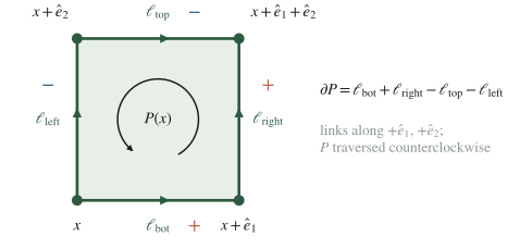
Figure 1. The oriented plaquette $P(x)$ and its boundary. Signs record whether a boundary link’s own orientation agrees (+) or disagrees (−) with the counterclockwise traversal.

2.2 Chains and $\partial$

A $p$-chain is a formal integer combination of oriented $p$-cells, $c={\sum }_i{n}_i{\sigma }_i$; they form the free abelian group $C_p(\Lambda ,\mathbb{Z})$. The boundary operator $\partial :C_p\to C_{p-1}$ assigns to each cell its oriented boundary:

$$\partial (\text{link }x\to x+\hat{\mu })=(x+\hat{\mu })-x,\partial P(x)={\ell }_{\mathrm{bot}}+{\ell }_{\mathrm{right}}-{\ell }_{\mathrm{top}}-{\ell }_{\mathrm{left}}$$

(Figure 1), and in general with signs $(-1{)}^{\text{position}}$ dictated by the ordered-tuple orientation.

The one identity everything rests on: ${\partial }^2=0$. Check it on Figure 1, symbol by symbol [Proved for the plaquette; the general case is the same cancellation]:

$$\partial (\partial P)=[(x+\hat{1})-x]+[(x+\hat{1}+\hat{2})-(x+\hat{1})]-[(x+\hat{1}+\hat{2})-(x+\hat{2})]-[(x+\hat{2})-x]=0.$$

Each corner appears exactly twice, once with each sign. “The boundary of a boundary is empty.”

3. Cochains and the coboundary operator

3.1 Cochains are fields

A $p$-cochain with coefficients in an abelian group $G$ is a $G$-valued function on oriented $p$-cells: $f\in C^p(\Lambda ,G)$, with $f(-\sigma )=-f(\sigma )$ under orientation reversal. This is exactly what a physicist means by a $p$-form field on the lattice:

cochain degree	field	examples in this course
0 (sites)	scalar	${\theta }_x$ (XY), heights $h$, dual photon $\sigma$
1 (links)	gauge field	$a_{\ell }$, the Villain integer $n_{\ell }$ (Week 3)
2 (plaquettes)	field strength / 2-form	$(da{)}_P$, vorticity, ${\mathbb{Z}}_N$ backgrounds $B$
3 (cubes)	3-form	monopole density $dn$ in gauge theory

Coefficients used: $\mathbb{Z}$, $\mathbb{R}$, $U(1)=\mathbb{R}/2\pi \mathbb{Z}$, ${\mathbb{Z}}_N$. The pairing of a cochain with a chain,

$$⟨f,c⟩=\sum _i{n}_{i}f({\sigma }_i)\text{for }c=\sum _i{n}_i{\sigma }_i,$$

is the lattice version of ${\int }_{c}f$.

3.2 The coboundary $d$: Stokes as a definition

Define $d:C^p\to C^{p+1}$ by declaring the discrete Stokes theorem to hold identically:

$$\boxed{⟨df,c⟩=⟨f,\partial c⟩\text{for all chains }c.}$$

Unpacked: $(df)$ on a $(p+1)$-cell is the signed sum of $f$ over that cell’s boundary. Concretely,

$$(d\phi )(x\to x+\hat{\mu })={\phi }_{x+\hat{\mu }}-{\phi }_x(\text{gradient}),(da)(P(x))=a_{\mathrm{bot}}+a_{\mathrm{right}}-a_{\mathrm{top}}-a_{\mathrm{left}}(\text{curl / field strength}),$$

and on 2-cochains, the signed sum over a cube’s six faces (divergence of a 2-form). Because ${\partial }^2=0$,

$$⟨d^{2}f,c⟩=⟨f,{\partial }^{2}c⟩=0\text{for all }c⟹\boxed{d^2=0.}$$

“Curl of a gradient vanishes”; “divergence of a curl vanishes”; the Bianchi identity — all of them are this one line, and on the lattice they are exact algebra, not smooth-function theorems.

Physical picture. The field strength $F=da$ of any lattice gauge field is automatically closed, $dF=0$ — Bianchi with no equations of motion invoked. So where do magnetic monopoles come from? From compactness: when the gauge field is an angle, the honest field strength is $F=da-2\pi n$ with an integer 2-cochain $n$ recording branch choices, and $dF=-2\pi dn$ need not vanish. The monopole density is literally $d^2$-of-a-multivalued-object — zero for a globally defined field, quantized and localized when the field is a chart. Weeks 8–11 are this sentence, unpacked with couplings attached.

3.3 The inner product and the codifferential

Give $C^p(\Lambda ,\mathbb{R})$ the inner product $⟨f,g⟩={\sum }_{p\text{-cells}}f(\sigma )g(\sigma )$. The codifferential $\delta :C^p\to C^{p-1}$ is the adjoint of $d$:

$$⟨\delta f,g⟩=⟨f,dg⟩\text{for all }g\in C^{p-1}.$$

Note that $\delta$ is the ${\ell }^2$ adjoint of $d$ with no further sign (conventions §2), so its form on a 1-cochain follows from one summation by parts. Writing $m_{\mu }(x)$ for the value of $m$ on the link ${\ell }_{\mu }(x)$ from $x$ to $x+\hat{\mu }$, and shifting $x\to x-\hat{\mu }$ in the first term (the torus has no boundary), we obtain

$$⟨m,dg⟩=\sum _{x,\mu }{m}_{\mu }(x)[g_{x+\hat{\mu }}-g_x]=\sum _x{g}_x\sum _{\mu }[m_{\mu }(x-\hat{\mu })-m_{\mu }(x)],$$

so that

$$(\delta m{)}_x=\sum _{\mu }[m_{\mu }(x-\hat{\mu })-m_{\mu }(x)]=\text{in}-\text{out},$$

the inflow minus the outflow at $x$. The physical divergence is therefore $-\delta m$. ${\delta }^2=0$ follows by adjointness. The lattice Laplacian is

$$\Delta =\delta d+d\delta \ge 0,$$

where positivity follows from $⟨f,\Delta f⟩=\Vert df{\Vert }^2+\Vert \delta f{\Vert }^2$. On 0-cochains $\delta f=0$ (there are no $(-1)$-cells), and the formula for $\delta$ applied to the 1-cochain $df$ gives

$$(\Delta f{)}_x=(\delta df{)}_x=\sum _{\mu }\left[\right(f_x-f_{x-\hat{\mu }})-(f_{x+\hat{\mu }}-f_x\left)\right]=\sum _{\mu }(2f_x-f_{x+\hat{\mu }}-f_{x-\hat{\mu }}),$$

the negative of the lattice second difference (the 5-point stencil in $d=2$ and the 7-point one in $d=3$, with the sign that makes it non-negative), as in conventions §2. Its kernel, the harmonic cochains, will turn out to be exactly the topology (§6).

4. Homology and cohomology, computed by hand

4.1 Definitions

• $f$ is closed if $df=0$; exact if $f=dg$. Exact ⟹ closed (since $d^2=0$).
• Cohomology: $H^p(\Lambda ,G)=\ker d{|}_{C^p}/\mathrm{im}d{|}_{C^{p-1}}$ — closed modulo exact.
• Homology: $H_p(\Lambda ,G)=\ker \partial {|}_{C_p}/\mathrm{im}\partial {|}_{C_{p+1}}$ — cycles modulo boundaries.

$H^p$ measures global field configurations: closed fields that are not the coboundary of anything — invisible to all local data, detectable only by integrating around non-contractible cycles.

Physical picture. In gauge-theory words: exact = pure gauge ($a=d\lambda$), closed = flat ($da=0$), and $H^1$ = flat-but-not-pure-gauge = the physically distinct Wilson-line holonomies around non-contractible loops. On a torus these are the moduli that label degenerate ground states of a topological phase (Semester II Week 2). Cohomology is not an abstraction bolted onto the physics; it is the count of vacua, and this week’s central skill is computing it.

4.2 The 2×2 torus, matrices displayed [Computed.]

We compute $H_{\bullet }(T^2,\mathbb{Z})$ on the smallest nontrivial lattice: the $2\times 2$ periodic square lattice. Cells: 4 sites $s_{ij}$, 8 links (4 $x$-links ${\ell }_{ij}^x$, 4 $y$-links ${\ell }_{ij}^y$), 4 plaquettes $P_{ij}$, indices $i,j\in \{0,1\}$ mod 2.

The matrix ${\partial }_1$ (8 columns = links, 4 rows = sites $s_{00},s_{10},s_{01},s_{11}$), from $\partial {\ell }_{ij}^x=s_{i+1,j}-s_{ij}$, $\partial {\ell }_{ij}^y=s_{i,j+1}-s_{ij}$:

$${\partial }_1=\left(\begin{array}{ccccccccc}& {\ell }_{00}^x& {\ell }_{10}^x& {\ell }_{01}^x& {\ell }_{11}^x& {\ell }_{00}^y& {\ell }_{10}^y& {\ell }_{01}^y& {\ell }_{11}^y\\ s_{00}& -1& +1& 0& 0& -1& 0& +1& 0\\ s_{10}& +1& -1& 0& 0& 0& -1& 0& +1\\ s_{01}& 0& 0& -1& +1& +1& 0& -1& 0\\ s_{11}& 0& 0& +1& -1& 0& +1& 0& -1\end{array}\right)$$

Each column sums to zero (every link has one head, one tail), so $\mathrm{rank}{\partial }_1\le 3$; and the three columns ${\ell }_{00}^x,{\ell }_{00}^y,{\ell }_{10}^y$ are visibly independent, so

$$\mathrm{rank}{\partial }_1=3,H_0=C_0/\mathrm{im}{\partial }_1={\mathbb{Z}}^4/{\mathbb{Z}}^3=\mathbb{Z}$$

— one connected component, as it must be. ($\mathrm{im}{\partial }_1$ = all site chains with total coefficient zero.)

The matrix ${\partial }_2$ (4 columns = plaquettes, 8 rows = links), from $\partial P_{ij}={\ell }_{ij}^x+{\ell }_{i+1,j}^y-{\ell }_{i,j+1}^x-{\ell }_{ij}^y$:

$${\partial }_2=\left(\begin{array}{ccccc}& P_{00}& P_{10}& P_{01}& P_{11}\\ {\ell }_{00}^x& +1& 0& -1& 0\\ {\ell }_{10}^x& 0& +1& 0& -1\\ {\ell }_{01}^x& -1& 0& +1& 0\\ {\ell }_{11}^x& 0& -1& 0& +1\\ {\ell }_{00}^y& -1& +1& 0& 0\\ {\ell }_{10}^y& +1& -1& 0& 0\\ {\ell }_{01}^y& 0& 0& -1& +1\\ {\ell }_{11}^y& 0& 0& +1& -1\end{array}\right)$$

Kernel of ${\partial }_2$: a combination $\sum c_{ij}{P}_{ij}$ has zero boundary iff (row ${\ell }_{00}^x$) $c_{00}=c_{01}$, (row ${\ell }_{10}^x$) $c_{10}=c_{11}$, (row ${\ell }_{00}^y$) $c_{00}=c_{10}$, (row ${\ell }_{01}^y$) $c_{01}=c_{11}$ — i.e. all $c_{ij}$ equal. So

$$\ker {\partial }_2=\mathbb{Z}\cdot (P_{00}+P_{10}+P_{01}+P_{11}),H_2=\ker {\partial }_2=\mathbb{Z},\mathrm{rank}{\partial }_2=4-1=3.$$

The generator of $H_2$ is the whole surface — the “volume cycle” of the torus.

$H_1$, the interesting one:

$$\dim \ker {\partial }_1=8-\mathrm{rank}{\partial }_1=5,\mathrm{rank}\mathrm{im}{\partial }_2=3⟹H_1\cong {\mathbb{Z}}^{5-3}={\mathbb{Z}}^2(\text{no torsion; see below}).$$

Explicit generators of the kernel: the two winding loops

$$A={\ell }_{00}^x+{\ell }_{10}^x(\text{around the }x\text{-direction}),B={\ell }_{00}^y+{\ell }_{01}^y(\text{around }y),$$

plus three plaquette boundaries $\partial P_{00},\partial P_{10},\partial P_{01}$. Modding out the boundaries leaves exactly $A$ and $B$:

$$\boxed{H_1(T^2,\mathbb{Z})=\mathbb{Z}[A]\oplus \mathbb{Z}[B].}$$

Torsion, systematically. The complete algorithm is the Smith normal form: any integer matrix $M$ can be brought to $\mathrm{diag}(d_1,d_2,\dots ,0,\dots )$ with $d_1\mid d_2\mid \cdots$ (the invariant factors) by invertible integer row/column operations, and

$$H_p\cong {\mathbb{Z}}^{n_p-r_p-r_{p+1}}\oplus \underset{i}{⨁}{\mathbb{Z}}_{d_i^{(p+1)}}(\text{over the invariant factors }{d}_i>1\text{ of }{\partial }_{p+1}),$$

with $n_p$ the number of $p$-cells and $r_p=\mathrm{rank}{\partial }_p$.

The reduction, performed. Run it on ${\partial }_2$ above; integer row/column operations only. Use column $P_{00}$ and its $+1$ in row ${\ell }_{00}^x$ as the first pivot: clear that row’s other entry by the column operation $P_{01}\to P_{01}+P_{00}$, then clear column $P_{00}$‘s remaining entries by row operations (${\ell }_{01}^x\to {\ell }_{01}^x+{\ell }_{00}^x$, ${\ell }_{00}^y\to {\ell }_{00}^y+{\ell }_{00}^x$, ${\ell }_{10}^y\to {\ell }_{10}^y-{\ell }_{00}^x$). The first row and column are now $(1,0,0,0)$. Repeat with the $+1$ of the reduced $P_{10}$ column (row ${\ell }_{10}^x$), then with the reduced $P_{01}$ column (its surviving $\pm 1$, e.g. in the modified ${\ell }_{01}^y$ row). After three pivots — each with pivot entry $\pm 1$, so each invariant factor is 1 — the fourth column has been emptied by the relation $P_{00}+P_{10}+P_{01}+P_{11}\mapsto 0$:

$$\mathrm{SNF}({\partial }_2)=\mathrm{diag}(1,1,1,0),\text{and identically}\mathrm{SNF}({\partial }_1)=\mathrm{diag}(1,1,1,0).$$

Feed the formula: $H_1={\mathbb{Z}}^{8-3-3}\oplus (\text{nothing, since all }{d}_i=1)={\mathbb{Z}}^2$, confirming the constructive computation. The algorithm is fully mechanical — this is the sense in which “computing the topology” is something one can hand to a computer algebra system, and the invariant factors are where any torsion would have announced itself.

Physical picture. What did the matrices just compute? $\ker {\partial }_1$ is the space of conserved currents on this lattice; $\mathrm{im}{\partial }_2$ is the subspace realizable as local eddies (plaquette circulations). The quotient — two surviving generators — says: on a torus there are exactly two ways for current to flow that no arrangement of local eddies can produce, the two global circulations. A superconducting loop’s persistent current modes, the winding sectors of Week 3, the flux sectors of a gauge theory on $T^2$: all are this quotient, computed once here with integer row reduction. When a topological-order paper says “the ground-state degeneracy is $|H_1(\Sigma ,{\mathbb{Z}}_N)|$,” this small linear algebra is the entire geometric content.

For our matrices all invariant factors equal 1, so no torsion appears — as befits the torus. A space where torsion does appear is the Klein bottle, $H_1(K,\mathbb{Z})=\mathbb{Z}\oplus {\mathbb{Z}}_2$: Problem 4 has you produce the invariant factor 2 by the same algorithm. Torsion is not exotica: ${\mathbb{Z}}_N$ gauge theories live on exactly this kind of arithmetic.

4.3 The general torus, the fast way [Computed.]

For $H^p(T^d)$ at any size, use the minimal cell structure: one $d$-cube with opposite faces identified. It has exactly $\left(\genfrac{}{}{0ex}{}{d}{p}\right)$ $p$-cells (one per choice of $p$ directions), and every boundary map vanishes, because under the identification each face of a cell occurs twice in its boundary, once from each side of the cube, with opposite signs. For the $1\times 1$ torus this is visible at once: each link has its head and its tail at the single site, $\partial \ell =x-x=0$, and the bottom and top edges of the plaquette are the same link, as are its left and right edges, so $\partial P={\ell }^x+{\ell }^y-{\ell }^x-{\ell }^y=0$. With $\partial =0$ and $d=0$, homology equals the chains and cohomology equals the cochains:

$$\boxed{H^p(T^d,G)\cong G^{\left(\genfrac{}{}{0ex}{}{d}{p}\right)},b_p=\left(\genfrac{}{}{0ex}{}{d}{p}\right).}$$

	$b_0$	$b_1$	$b_2$	$b_3$	$b_4$
$T^2$	1	2	1	—	—
$T^3$	1	3	3	1	—
$T^4$	1	4	6	4	1

With $G={\mathbb{Z}}_N$: $H^1(T^d,{\mathbb{Z}}_N)={\mathbb{Z}}_N^d$, the counting that becomes $\mathrm{GSD}=N^{2g}$ for ${\mathbb{Z}}_N$ gauge theory on a genus-$g$ surface (Semester II Week 2), and $H^2(T^4,{\mathbb{Z}}_N)={\mathbb{Z}}_N^6$, the space of ‘t Hooft-flux backgrounds in Semester II Week 6.

Why the fine $2\times 2$ answer and the minimal answer agree [Sketched.]: homology is a homotopy invariant — refining a cell decomposition does not change it. The mechanism, without the machinery: subdividing a cell adds equal numbers of new generators and new relations (each new face is killed by a new boundary), so kernels-mod-images are unchanged; the formal proof organizes this bookkeeping into chain homotopies, which we state and do not need [named gap; Nakahara §3.3]. Operationally: compute on the coarsest complex available; put fields on the finest.

5. The dual lattice

5.1 Construction and the degree flip

The dual lattice ${\Lambda }^{\ast }$ places a site at the center of each $d$-cell of $\Lambda$; in general,

$$p\text{-cell of }\Lambda ⟷(d-p)\text{-cell of }{\Lambda }^{\ast }(\text{the unique dual cell it pierces}).$$

Figure 2 draws the two lattices in $d=2$.

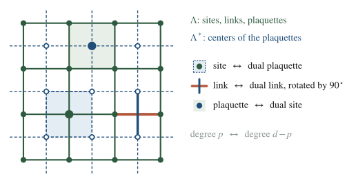
Figure 2. Direct and dual lattices in $d=2$. Every object of degree $p$ has a shadow of degree $d-p$.

In $d=3$: sites↔cubes, links↔plaquettes, plaquettes↔links, cubes↔sites. In $d=4$: plaquettes↔plaquettes — degree 2 is self-dual, the structural reason electric–magnetic duality is special to four dimensions (Week 8).

5.2 $\delta =-\star d\star$ on 1-cochains, verified in $d=2$ [Computed.]

The Hodge map $\star :C^p(\Lambda )\to C^{d-p}({\Lambda }^{\ast })$ transports the value of a cochain on a $p$-cell to the dual $(d-p)$-cell, with the sign of a shuffle. Write a $p$-cell as $(x;S)$, with $x$ its base site and $S=\{{\mu }_1<\cdots <{\mu }_p\}$ its directions, $S^c$ for the complementary directions and ${\hat{e}}_S={\sum }_{\mu \in S}\hat{\mu }$. Following conventions §2, the dual of $(x;S)$ is the $(d-p)$-cell of ${\Lambda }^{\ast }$ based at $x+\frac{1}{2}{\hat{e}}_S-\frac{1}{2}{\hat{e}}_{S^c}$ and spanned by $S^c$ in increasing order, and

$$(\star f)((x;S{)}^{\ast })=ϵ(S,S^c)f((x;S)),$$

where $ϵ(S,S^c)$ is the sign of the permutation that sorts the sequence $(S,S^c)$; the same rule maps ${\Lambda }^{\ast }$ back to $\Lambda$. With this sign, exactly as for differential forms in the continuum,

$$\star \star =(-1{)}^{p(d-p)},\delta =(-1{)}^{d(p+1)+1}\star d\star \text{on }{C}^p,$$

identities that conventions §2 records after checking them cell by cell on the lattice for every $p$ in $d=2,3,4$. In $d=2$ on 1-cochains the sign is $(-1{)}^{2\cdot 2+1}=-1$, so $\delta =-\star d\star$, and we now verify this case by hand.

In $d=2$ the rule rotates a link by $+90°$. The dual of ${\ell }_1(x)$, with $ϵ(1,2)=+1$, is the dual link from $x+(\frac{1}{2},-\frac{1}{2})$ to $x+(\frac{1}{2},\frac{1}{2})$ carrying $m_1(x)$; the dual of ${\ell }_2(x)$, with $ϵ(2,1)=-1$, is the dual link from $x+(-\frac{1}{2},\frac{1}{2})$ to $x+(\frac{1}{2},\frac{1}{2})$ carrying $-m_2(x)$, which is the same as the link from $x+(\frac{1}{2},\frac{1}{2})$ to $x+(-\frac{1}{2},\frac{1}{2})$ carrying $+m_2(x)$. The dual of the site $x$ ($S=\varnothing$, $ϵ=+1$) is the dual plaquette $x^{\ast }$ based at $x-(\frac{1}{2},\frac{1}{2})$, oriented counter-clockwise, and its four edges are the duals of the four links at $x$. Reading off the positions, the right and top edges of $x^{\ast }$ are the duals of the outgoing links ${\ell }_1(x)$ and ${\ell }_2(x)$, and the left and bottom edges are the duals of the incoming links ${\ell }_1(x-\hat{1})$ and ${\ell }_2(x-\hat{2})$. With the boundary signs of Figure 1,

$$\begin{array}{rl}(d\star m)(x^{\ast })& =\star m(\text{bottom})+\star m(\text{right})-\star m(\text{top})-\star m(\text{left})\\ & =-m_2(x-\hat{2})+m_1(x)+m_2(x)-m_1(x-\hat{1})\\ & =m({\ell }_{x,\mathrm{out}}^{(1)})+m({\ell }_{x,\mathrm{out}}^{(2)})-m({\ell }_{x,\mathrm{in}}^{(1)})-m({\ell }_{x,\mathrm{in}}^{(2)})\\ & =-(\delta m{)}_x,\end{array}$$

where the last step is the in-minus-out form of $\delta$ derived in §3.3. That is, the $+90°$ rotation sends the dual links of the two outgoing links along the counter-clockwise boundary of $x^{\ast }$ and those of the two incoming links against it, so that $(d\star m)(x^{\ast })=\text{out}-\text{in}$. Mapping back with $\star :C^2({\Lambda }^{\ast })\to C^0(\Lambda )$, where $ϵ(\{1,2\},\varnothing )=+1$, gives $\star d\star m=-\delta m$, the case $d=2$, $p=1$ of the general formula. One picture is worth the index chase: rotating a vector field by 90° turns its divergence into a curl, and the lattice version of that freshman fact is the entire content of $\delta =-\star d\star$ here.

5.3 Poincaré duality

$$\boxed{H^p(T^d,G)\cong H_{d-p}(T^d,G).}$$

A closed $p$-cochain on $\Lambda$ is a $(d-p)$-cycle on ${\Lambda }^{\ast }$ (transport by $\star$; closedness becomes cycle-ness by §5.2). Check against §4: $H^1(T^2)={\mathbb{Z}}^2=H_1(T^2)$ ✓. The physical payoff is the defect-geometry flip: a defect defined by a $(p+1)$-cochain equation $dn\ne 0$ lives on a $(d-p-1)$-cycle of the dual lattice:

object	cochain eq.	$d=2$	$d=3$	$d=4$
vortex of a compact scalar	$v=dn,n\in C^1$	point	line	sheet
monopole of a compact gauge field	$m=dn,n\in C^2$	—	point (instanton)	worldline

The boxed row of Block C: the same equation $dn$, read in $d=3$ vs $d=4$, gives Polyakov’s instanton plasma vs the dual superconductor’s loop condensate. Geometry, not dynamics, makes them different problems.

6. Hodge theory: harmonic = topological [Proved.]

Theorem (discrete Hodge decomposition). On a finite complex, with the inner product of §3.3,

$$C^p=\mathrm{im}d\oplus \mathrm{im}\delta \oplus {\mathcal{H}}^p,{\mathcal{H}}^p\equiv \ker \Delta {|}_{C^p}=\{h:dh=0\text{ and }\delta h=0\},$$

orthogonal direct sum, and ${\mathcal{H}}^p\cong H^p(\Lambda ,\mathbb{R})$; in particular $\dim \ker \Delta {|}_{C^p}=b_p$.

Proof. (i) Orthogonality: $⟨d\alpha ,\delta \beta ⟩=⟨d(d\alpha ),\beta ⟩=0$ by $d^2=0$ and adjointness. (ii) Harmonic ⟺ closed and co-closed: $⟨h,\Delta h⟩=⟨h,\delta dh⟩+⟨h,d\delta h⟩=\Vert dh{\Vert }^2+\Vert \delta h{\Vert }^2$, so $\Delta h=0$ iff both vanish. (iii) The complement: $h\perp \mathrm{im}d⟺⟨h,d\alpha ⟩=⟨\delta h,\alpha ⟩=0\forall \alpha ⟺\delta h=0$; likewise $h\perp \mathrm{im}\delta ⟺dh=0$. So $(\mathrm{im}d\oplus \mathrm{im}\delta {)}^{\perp }={\mathcal{H}}^p$, giving the decomposition (finite dimensions: orthogonal complement always splits). (iv) Harmonics compute cohomology: let $f$ be closed and decompose $f=d\alpha +\delta \beta +h$. Then $0=df=d\delta \beta$, so $0=⟨d\delta \beta ,\beta ⟩=\Vert \delta \beta {\Vert }^2$ and the coexact piece vanishes: every closed $f$ is (exact) + (harmonic), and the harmonic part is unique in its class ($h-h^{\prime }=d\alpha$ with both harmonic ⟹ $\Vert d\alpha {\Vert }^2=⟨h-h^{\prime },d\alpha ⟩=⟨\delta (h-h^{\prime }),\alpha ⟩=0$). Thus ${\mathcal{H}}^p\cong H^p$. $\square$

Worked: the harmonic 1-cochains of $T^2$ [Computed.] Take $h^{(x)}$ = value 1 on every $x$-link, 0 on every $y$-link. Then $(d{h}^{(x)})(P)=1+0-1-0=0$ on every plaquette (Figure 1’s signs), and $(\delta h^{(x)}{)}_x=1-1=0$ at every site (one incoming, one outgoing $x$-link). Harmonic. Likewise $h^{(y)}$. These two span ${\mathcal{H}}^1$: $\dim =b_1=2$ ✓ — the two “constant winds” around the torus, the zero modes of the Laplacian, the flat connections. Topology as the kernel of a matrix you can diagonalize.

Physical picture. Hodge is the statement that every field configuration splits into gauge junk + local physics + topology: $f=d\alpha$ (pure gauge / gradient part) $+\delta \beta$ (the part sourced by local currents) $+h$ (the finitely many global modes no local operation reaches). In Week 3 exactly this split separates spin waves ($\delta \beta$-type fluctuations) from winding sectors ($h$) and lets the vortices be counted cleanly; the zero mode that enforces charge neutrality in the Coulomb gas is the $b_0=1$ harmonic constant on the dual lattice. When a numerical collaborator says “we fix the zero modes,” this decomposition is what they are fixing.

7. Poisson resummation on cochains: the duality engine

7.1 The identity, proved [Model proof.]

Claim: for $f$ Schwartz (rapid decay suffices),

$$\sum _{n\in \mathbb{Z}}f(n)=\sum _{w\in \mathbb{Z}}{\int }_{-\infty }^{\infty }dxf(x)e^{2\pi iwx}.$$

Proof. The Dirac comb $\text{Sha}(x)={\sum }_n\delta (x-n)$ is periodic with period 1, so it has a Fourier series $\text{Sha}(x)={\sum }_w{c}_w{e}^{2\pi iwx}$ with

$$c_w={\int }_0^1\text{Sha}(x)e^{-2\pi iwx}dx=e^{-2\pi iw\cdot 0}=1$$

(exactly one delta, at $x=0$, sits in the fundamental domain). Thus $\text{Sha}={\sum }_w{e}^{2\pi iwx}$ as tempered distributions, and integrating $f$ against both sides gives the claim; Schwartz decay justifies the interchanges [named gap: distributional convergence, standard]. $\square$

The Gaussian case was derived independently in Week 1 §6 by the method of images — same identity, mechanism attached.

7.2 The recipe (memorize)

Every abelian duality in this course is the following four moves, applied to an integer cochain (the engine fires in Week 3, Week 8, and — made exact — in Semester II Week 12):

1. Villain form: write the compact theory with an explicit integer $p$-cochain $n$.
2. Poisson-resum $n$ (one comb per cell): a dual integer variable appears, one per dual $(d-p)$-cell.
3. Integrate the original field: it now appears linearly; integrating it out imposes a constraint (current conservation, $\delta (\cdot )=0$) on the dual variable.
4. Solve the constraint exactly, with the toolkit of this week: transported by $\star$ (§5.2), the co-closed integer variable becomes a closed integer cochain on ${\Lambda }^{\ast }$, and on the torus every closed integer cochain is the coboundary of an integer dual potential plus an integer combination of fixed unit-winding representatives, one for each generator of the cohomology. The constraint has no exceptions, so no defect survives this step: in Week 3 the conserved current becomes integer heights plus two winding sectors. The defects of the original theory reappear only at a second Poisson resummation, when the integer dual potential is traded for a real field and the new integers conjugate to it turn out to be the defect charges (the heights of Week 3 §3, resummed in Week 3 §4, give the vortices).

Steps 3–4 are where §§5–6 earn their keep: “solve $\delta m=0$” means “transport by $\star$, split the closed result into an exact and a topological part as in §6, and keep track of the $b_p$ winding sectors”, with integer unit-winding representatives in place of the real harmonic ones (Week 3 §3).

8. The intersection pairing: one integer, seed of a Hilbert space

On $T^2$, the two homology generators $A$ (the $x$-winding loop) and $B$ (the $y$-winding loop) intersect once:

$$A\cdot A=0,B\cdot B=0,A\cdot B=1.$$

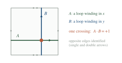
Figure 3. The intersection form of the torus. This single “+1” is the origin of the clock–shift algebra.

Signed intersection counting extends to a bilinear pairing $H_p\times H_{d-p}\to \mathbb{Z}$ (or ${\mathbb{Z}}_N$) on any $T^d$; it is the homological face of the linking of operators in spacetime. Preview of its operator life [Heuristic here; derived in Semester II Week 2]: in ${\mathbb{Z}}_N$ gauge theory, let $Z$ = the operator measuring the holonomy along $A$, and $X$ = the operator that shifts that holonomy (equivalently, measures/creates flux along $B$). Because $B$ must cross $A$ exactly once to close, reordering the two operations differs by one unit of ${\mathbb{Z}}_N$ phase:

$$ZX=\omega XZ,\omega =e^{2\pi i/N}.$$

Since the holonomy is an element of ${\mathbb{Z}}_N$, the operator $Z={\omega }^{\text{holonomy}}$ obeys $Z^N=1$, and shifting the holonomy $N$ times returns it, $X^N=1$. With $Z$ and $X$ unitary and $Z^N=X^N=1$, this clock–shift algebra has a unique irreducible representation, of dimension $N$ [Proved.]. Because $Z^N=1$, $Z$ is diagonalizable with eigenvalues among the $N$-th roots of unity; let $v$ be a unit eigenvector, $Zv=\lambda v$. The relation $ZX=\omega XZ$ gives $Z(X^{k}v)={\omega }^k\lambda X^{k}v$, so $v,Xv,\dots ,X^{N-1}v$ are unit vectors ($X$ is unitary) and eigenvectors of $Z$ with the $N$ distinct eigenvalues ${\omega }^k\lambda$, and therefore orthonormal. Their span $V_v$ is invariant under $Z$, because each of them is an eigenvector, and under $X$, because $X(X^{N-1}v)=X^{N}v=v$; this cyclic subspace is where $X^N=1$ enters. Irreducibility forces $V_v$ to be the whole space, which is therefore $N$-dimensional. Its $Z$-eigenvalues are all $N$ roots of unity, so we may choose $v$ with $\lambda =1$, and then in the basis $e_k=X^{k}v$

$$Z{e}_k={\omega }^k{e}_k,X{e}_k=e_{k+1(\mathrm{mod}N)},$$

the clock and shift matrices; any two irreducible representations are thus unitarily equivalent, by $e_k\mapsto e_k^{\prime }$. (Without $X^N=1$ we would only know, by Schur’s lemma, that $X^N=c1$ with $|c|=1$, since $X^N$ commutes with $Z$ and with $X$, and each value of $c$ gives an inequivalent representation.) Any theory realizing the algebra on its ground states therefore has $N$-fold degeneracy per conjugate cycle pair.

On a genus-$g$ surface the intersection form has a symplectic normal form: $2g$ cycle generators $A_1,B_1,\dots ,A_g,B_g$ with $A_i\cdot B_j={\delta }_{ij}$ and all other intersections zero. Now count operators in a ${\mathbb{Z}}_N$ gauge theory, which carries two species of loop operator — electric (Wilson) and magnetic (dual/‘t Hooft) lines, both wrappable on any cycle. The pairs (electric on $A_i$, magnetic on $B_i$) and (electric on $B_i$, magnetic on $A_i$) each realize one clock–shift algebra, they mutually commute (their cycles either coincide in species or intersect evenly), and no other independent pair exists: two algebras per handle, and therefore ground-state dimension $N^2$ per handle,

$$\mathrm{GSD}=N^{2g}.$$

Two assumptions entered that count, and both are theory-dependent: that the ground-state algebra is generated by the two loop species, and that no relation collapses it — both established for ${\mathbb{Z}}_N$ gauge theory in its deconfined phase in Semester II Week 2, where the operators are constructed. The homological input — the symplectic basis and one “+1” per handle — is complete here. That is topological order’s ground-state count, and its entire kinematic origin is Figure 3.

9. Cup product: a first meeting [Computed in low degree.]

Semester II needs one more operation, the cup product $\cup :C^p\times C^q\to C^{p+q}$, which is the lattice version of the wedge product. We use the cubical product fixed in conventions §8: for $\alpha \in C^p$, $\beta \in C^q$ and a $(p+q)$-cell $(x;S)$, in the notation of §5.2,

$$(\alpha \cup \beta )(x;S)=\sum _{\begin{array}{c}A\subset S\\ |A|=p\end{array}}ϵ(A,S\setminus A)\alpha (x;A)\beta (x+{\hat{e}}_A;S\setminus A),$$

where the sum runs over the ways of splitting the directions of the cell into a set $A$ for $\alpha$ and its complement $S\setminus A$ for $\beta$, and $ϵ(A,S\setminus A)$ is the sign of the shuffle that sorts $(A,S\setminus A)$, the same sign as in the Hodge map. Thus $\alpha$ is evaluated on the face spanned by $A$ at the base corner $x$, and $\beta$ on the complementary face at the corner $x+{\hat{e}}_A$ that we reach by walking along $A$. (Chen–Tata, arXiv:2106.05274, §V, construct the same product with the two factors written in the opposite order, $\alpha {\cup }_{\mathrm{CT}}\beta =(-1{)}^{pq}\beta \cup \alpha$, and with it the higher cup products ${\cup }_k$ that Semester II uses.)

In low degree the formula gives the rules we compute with. For a 0-cochain $f$ the only split gives all the directions of the cell to the other factor, so for a 1-cochain $\beta$ on a link $\ell$ and a 2-cochain $\omega$ on a plaquette $P_{\mu \nu }(x)$

$$\begin{array}{rlrl}(f\cup \beta )(\ell )& =f(\text{tail})\beta (\ell ),& (\beta \cup f)(\ell )& =\beta (\ell )f(\text{head}),\\ (f\cup \omega )(P_{\mu \nu }(x))& =f(x)\omega (P),& (\omega \cup f)(P_{\mu \nu }(x))& =\omega (P)f(x+\hat{\mu }+\hat{\nu })\end{array}$$

(“front value” against “back value”). For two 1-cochains on a plaquette there are two splits, $A=\{\mu \}$ with $ϵ(\mu ,\nu )=+1$ and $A=\{\nu \}$ with $ϵ(\nu ,\mu )=-1$, and the rule has two terms,

$$(\alpha \cup \beta )(P_{\mu \nu }(x))={\alpha }_{\mu }(x){\beta }_{\nu }(x+\hat{\mu })-{\alpha }_{\nu }(x){\beta }_{\mu }(x+\hat{\nu })(\mu <\nu ),$$

where ${\alpha }_{\mu }(x)=\alpha ({\ell }_{\mu }(x))$ as in §3.3. On the plaquette of Figure 1 this reads $(\alpha \cup \beta )(P)={\alpha }_{\mathrm{bot}}{\beta }_{\mathrm{right}}-{\alpha }_{\mathrm{left}}{\beta }_{\mathrm{top}}$: each of the two lattice paths from $x$ to $x+\hat{1}+\hat{2}$ contributes $\alpha$ on its first leg times $\beta$ on its second leg, the lower path with a plus sign and the upper path with a minus sign. Both terms are needed, as the next computation shows.

Leibniz [Computed.]. We check $d(f\cup \beta )=df\cup \beta +f\cup d\beta$ on the plaquette $P(x)$ of Figure 1, the case $p=0$ of

$$d(\alpha \cup \beta )=d\alpha \cup \beta +(-1{)}^p\alpha \cup d\beta .$$

The left side is the signed boundary sum of $(f\cup \beta )(\ell )=f(\text{tail}(\ell ))\beta (\ell )$, and the tails of ${\ell }_{\mathrm{bot}},{\ell }_{\mathrm{right}},{\ell }_{\mathrm{top}},{\ell }_{\mathrm{left}}$ are $x$, $x+\hat{1}$, $x+\hat{2}$, $x$, so

$$d(f\cup \beta )(P)=f(x){\beta }_{\mathrm{bot}}+f(x+\hat{1}){\beta }_{\mathrm{right}}-f(x+\hat{2}){\beta }_{\mathrm{top}}-f(x){\beta }_{\mathrm{left}}.$$

On the right side the two-term rule gives $(df\cup \beta )(P)=df({\ell }_{\mathrm{bot}}){\beta }_{\mathrm{right}}-df({\ell }_{\mathrm{left}}){\beta }_{\mathrm{top}}$, with $df({\ell }_{\mathrm{bot}})=f(x+\hat{1})-f(x)$ and $df({\ell }_{\mathrm{left}})=f(x+\hat{2})-f(x)$, and the $0\cup 2$ rule gives $(f\cup d\beta )(P)=f(x)(d\beta )(P)$. The eight terms are

$$\begin{array}{rl}(df\cup \beta )(P)+(f\cup d\beta )(P)& =f(x+\hat{1}){\beta }_{\mathrm{right}}-f(x){\beta }_{\mathrm{right}}-f(x+\hat{2}){\beta }_{\mathrm{top}}+f(x){\beta }_{\mathrm{top}}\\ & +f(x){\beta }_{\mathrm{bot}}+f(x){\beta }_{\mathrm{right}}-f(x){\beta }_{\mathrm{top}}-f(x){\beta }_{\mathrm{left}}\\ & =f(x){\beta }_{\mathrm{bot}}+f(x+\hat{1}){\beta }_{\mathrm{right}}-f(x+\hat{2}){\beta }_{\mathrm{top}}-f(x){\beta }_{\mathrm{left}},\end{array}$$

where the two terms in $f(x){\beta }_{\mathrm{right}}$ and the two in $f(x){\beta }_{\mathrm{top}}$ cancel, and the four survivors are, term by term, the left side. Leibniz holds exactly. Note that the second term of the $1\cup 1$ rule is indispensable: without it the right side would lack $-df({\ell }_{\mathrm{left}}){\beta }_{\mathrm{top}}$, and the two sides would differ by $[f(x)-f(x+\hat{2})]{\beta }_{\mathrm{top}}$ on the top link of every plaquette. In general degree the rule is proved by Chen–Tata (Prop. 3) for their ordering, and ours inherits it, since the opposite product of a product that obeys Leibniz obeys the same rule [Stated — refs: Chen–Tata]; conventions §8 also records a cell-by-cell check on random integer cochains for every degree pair up to $d=5$. Problem 5⋆(a) repeats the audit for two 1-cochains on a cube, where the sign $(-1{)}^p$ first bites.

The continuum limit [Computed.]. For constant 1-cochains, ${\alpha }_{\mu }(x)={\alpha }_{\mu }$ and ${\beta }_{\mu }(x)={\beta }_{\mu }$, the two-term rule gives

$$(\alpha \cup \beta )(P_{12})={\alpha }_1{\beta }_2-{\alpha }_2{\beta }_1=(\alpha \wedge \beta {)}_{12}$$

exactly, so the cup product itself reproduces the wedge, and for constant fields $\beta \cup \alpha =-\alpha \cup \beta$ holds on the nose. For varying fields we regroup the four terms of the symmetric combination, which graded commutativity would set to zero, as

$$(\alpha \cup \beta +\beta \cup \alpha )(P_{\mu \nu }(x))={\alpha }_{\mu }(x){\nabla }_{\mu }{\beta }_{\nu }(x)-{\beta }_{\nu }(x){\nabla }_{\nu }{\alpha }_{\mu }(x)+{\beta }_{\mu }(x){\nabla }_{\mu }{\alpha }_{\nu }(x)-{\alpha }_{\nu }(x){\nabla }_{\nu }{\beta }_{\mu }(x),$$

where ${\nabla }_{\mu }g(x)=g(x+\hat{\mu })-g(x)$ is the forward difference. Every term contains a lattice difference of a field, so the non-commutativity enters only through the variation of the fields from site to site, and for fields that vary slowly on the lattice scale it is suppressed by one power of $a_0$ relative to $\alpha \wedge \beta$.

Graded commutativity. On the lattice $\alpha \cup \beta \ne (-1{)}^{pq}\beta \cup \alpha$ in general, and the failure is physical. In the lowest degree the two rules for a 0-cochain and a 1-cochain give, on any link,

$$(f\cup \beta -\beta \cup f)(\ell )=[f(\text{tail})-f(\text{head})]\beta (\ell )=-(df)(\ell )\beta (\ell ),$$

a product of two 1-cochains on the same link. On a link the higher cup product ${\cup }_1$ of two 1-cochains is exactly such a product of values, and ${\cup }_1$ vanishes when either factor is a 0-cochain, so this is the degree-$(0,1)$ instance of the term $df{\cup }_1\beta$ of the general statement, whose sign is fixed together with ${\cup }_1$. For cocycles the difference is a coboundary,

$$\alpha \cup \beta -(-1{)}^{pq}\beta \cup \alpha =\pm d(\alpha {\cup }_1\beta )(d\alpha =d\beta =0),$$

while for general cochains the right side acquires the extra terms $d\alpha {\cup }_1\beta$ and $\alpha {\cup }_{1}d\beta$; the signs are those of Chen–Tata eq. (29), adopted when ${\cup }_1$ is first used in Semester II Weeks 6–7 (conventions §8) [Stated — refs: Chen–Tata]. Two consequences matter already.

First, on cohomology classes the product is graded-commutative, since the defect is a coboundary; in particular its sum over a closed surface vanishes. We check this on the $L\times L$ torus with the harmonic 1-cochains of §6 [Computed.]. Because $h^{(x)}$ vanishes on $y$-links and $h^{(y)}$ on $x$-links, only one of the two terms survives on each plaquette,

$$(h^{(x)}\cup h^{(y)})(P_{12}(x))=h_1^{(x)}(x)h_2^{(y)}(x+\hat{1})=1,(h^{(y)}\cup h^{(x)})(P_{12}(x))=-h_2^{(y)}(x)h_1^{(x)}(x+\hat{2})=-1,$$

and summing over the $L^2$ plaquettes,

$$\sum _P{h}^{(x)}\cup h^{(y)}=L^2,\sum _P{h}^{(y)}\cup h^{(x)}=-L^2.$$

On the winding loops $A$ and $B$ of §4.2 (on the $L\times L$ torus, a row of $L$ $x$-links and a column of $L$ $y$-links) the classes have windings $⟨h^{(x)},A⟩=⟨h^{(y)},B⟩=L$, so the normalized classes $[h^{(x)}/L]$ and $[h^{(y)}/L]$ are dual to $A$ and $B$, and their cup-product pairing is the antisymmetric matrix $\left(\begin{array}{cc}0& 1\\ -1& 0\end{array}\right)$. This is the matrix of the intersection form of §8 in the basis $(A,B)$, with $B\cdot A=-A\cdot B=-1$ because intersections of 1-cycles on a surface are antisymmetric. With the first term of the $1\cup 1$ rule alone, the second sum would come out $0$ and the intersection form would be lost.

Second, at the cochain level the correction carries physics. The controlled non-commutativity carries the ‘t Hooft anomalies of Semester II Week 6, where the Pontryagin square $\mathcal{P}(B)$ is built exactly from $B\cup B$ and $B{\cup }_{1}dB$. For this reason we never simplify cup products by pretending that they commute.

10. Subtleties and fine print

F1 — Orientations are chosen once, then never renegotiated. Every sign in $\partial$, $d$, $\delta$, $\star$, and $\cup$ descends from the single global orientation convention of §2.1. Mid-calculation re-derivations of signs are the leading cause of “duality off by a sign” errors; the professional habit is to fix conventions (ours: conventions §§1–2 for $\partial$, $d$, $\delta$ and $\star$, §8 for $\cup$) and transport signs, never re-decide them.

F2 — Coarse for topology, fine for fields. Homology is homotopy-invariant (§4.3), so compute it on the minimal complex; but fields (cochains with actions) live on the fine lattice, where entropy and local dynamics reside. The two-lattice discipline — count global sectors coarsely, integrate fluctuations finely — is exactly how Week 3 separates winding sectors from spin waves.

F3 — Torsion exists, and ${\mathbb{Z}}_N$ physics feels it. On $T^d$ all homology is free, but on non-orientable or twisted spaces invariant factors $>1$ appear ($H_1(\text{Klein})=\mathbb{Z}\oplus {\mathbb{Z}}_2$, Problem 4). Then coefficients matter: $H^p(X,{\mathbb{Z}}_N)$ is not just ”$b_p$ copies of ${\mathbb{Z}}_N$” — torsion contributes extra pieces (universal-coefficient bookkeeping [Stated — refs: Nakahara §3.4]). ${\mathbb{Z}}_N$ gauge theories on such spaces have ground-state counts sensitive to this arithmetic; on tori we are safe, and we will say so whenever we use it.

F4 — The dual lattice is a different complex, not a shifted copy. Objects do not “also live” on ${\Lambda }^{\ast }$; they live on $\Lambda$ or on ${\Lambda }^{\ast }$, and $\star$ is a map, with orientation content (§5.2’s sign), between the two. Monopoles are dual-lattice objects, full stop; drawing both lattices (Figure 2) before any duality computation prevents the most common category error in this subject.

F5 — Boundary conditions are part of the complex. Everything above assumed the torus. Open boundaries change $H_{\bullet }$ (relative homology enters), and physical statements like “neutrality is enforced by the zero mode” depend on it. The course works on $T^d$ by default precisely to keep the harmonic bookkeeping clean; when a result depends on that choice we flag it.

F6 — Cohomology with compact coefficients has its own integers. A $U(1)$-valued cochain is not an $\mathbb{R}$-valued one: closedness mod $2\pi$, not closedness, is the gauge-invariant statement, and the integer “branch sheets” ($n$ in the Villain form) are exactly the difference. The clean formalization — $U(1)\cong \mathbb{R}/2\pi \mathbb{Z}$ cochains ↔ pairs $(\mathbb{R}\text{-cochain},\mathbb{Z}\text{-cochain})$ — is the Villain substitution of Week 3.

11. Common misconceptions

• ”$d$ is a finite-difference approximation to the continuum derivative.” No: on the lattice, $d$, ${\partial }^2=0$, Stokes, and Bianchi are exact. The continuum is the limit of the lattice here, not the other way around; nothing this week has discretization error.
• “Homology depends on which lattice/triangulation you chose.” It does not (§4.3) — that invariance is precisely why it deserves the name topology and why the $2\times 2$ computation of §4.2 already gives the answer for every size.
• “The dual lattice is just the original shifted by half a lattice spacing.” Its sites are; the structure is not — degrees flip ($p\leftrightarrow d-p$), orientations transform, and divergences become curls (§5.2). Treating ${\Lambda }^{\ast }$ as a shifted $\Lambda$ collapses the distinction that makes electric–magnetic duality nontrivial.

12. What to take away

1. Fields are cochains; $d$ is Stokes-by-definition; $d^2=0$ is Bianchi. Gradient, curl, and divergence are one operator in three degrees, exactly, with no continuum limit taken.
2. Topology is finite linear algebra. $H_{\bullet }(T^2)$ computed from two displayed integer matrices; $H^p(T^d,G)=G^{\left(\genfrac{}{}{0ex}{}{d}{p}\right)}$ from the minimal complex; Smith normal form as the general algorithm, torsion included.
3. Hodge splits every field into gauge + local + global [Proved], and the global (harmonic) part has dimension $b_p$ — topology as the kernel of a Laplacian. This split is the anatomy of every duality ahead.
4. The dual lattice flips degree, turning defect equations $dn\ne 0$ into points, lines, or sheets depending on $d$ — the single fact that organizes Block C.
5. One intersection number ($A\cdot B=1$) seeds the clock–shift algebra and therefore the ground-state degeneracy of topological order; the cup product’s controlled non-commutativity will carry the anomalies. The kinematics of Semester II is already on this page.

13. Looking ahead: Week 3

The engine is assembled: Villain form (integer cochains), Poisson resummation (proved), Hodge (proved), dual lattice (built). Week 3 fires it at the 2d XY model and carries the José–Kadanoff–Kirkpatrick–Nelson duality through with every constant on the page: the exact rewriting into a height model, the second resummation producing spin waves and vortex charges, the zero mode enforcing neutrality, the lattice Green function constant of Week 1 becoming the vortex fugacity — ending at the Coulomb gas whose unbinding, in Week 4, is BKT.

14. Problem set

Problems 1–3 are the classroom core and use only §§3–6; Problems 4⋆, 5⋆, 6⋆ and 8⋆ are self-study consolidation, solvable from the note, each with a hint or an indicated method; Problem 7⋆⋆ is a research extension and states what is known, what is explored and what counts as completion.

Core problems (everyone).

1. Boundary matrices on $T^2$, size $3\times 3$. Repeat §4.2 on the $3\times 3$ torus far enough to confirm $\mathrm{rank}{\partial }_1=8$, $\dim \ker {\partial }_2=1$, and $H_1={\mathbb{Z}}^2$ again. (Set up the matrices; compute ranks by exhibiting pivots, not by brute force.) Where in your computation is homotopy invariance visible?

2. Cohomology of $T^3$. (a) On the minimal complex of $T^3$, list the cells, confirm all boundary maps vanish, and read off $b_p=(1,3,3,1)$. (b) On a fine $L^3$ lattice, exhibit explicit generators: the three winding 1-cochains and the three “sheet” 2-cochains, and verify closedness and non-exactness of each. (c) Verify Poincaré duality $H^1\cong H_2$ by matching your generators across the dual lattice.

3. Laplacian zero modes. (a) Write $\Delta$ on 0-cochains of the $2\times 2$ torus as an explicit $4\times 4$ matrix and confirm its kernel is the constants ($b_0=1$). (b) Verify that $h^{(x)},h^{(y)}$ of §6 are annihilated by the 1-cochain Laplacian ${\Delta }_1=\delta d+d\delta$ (compute both terms separately).

Starred problems (self-study consolidation).

4⋆. Torsion: the Klein bottle. Build the minimal cell complex of the Klein bottle: one site, two links $a,b$, one 2-cell glued along the edge word $aba{b}^{-1}$ (the orientation-reversing identification). Show $\partial P=2a$ directly from the edge word, write ${\partial }_2$ as a $2\times 1$ integer matrix, compute its Smith normal form, extract the invariant factor 2, and conclude $H_1=\mathbb{Z}\oplus {\mathbb{Z}}_2$. Then compute $H^1(K,{\mathbb{Z}}_2)$ and note it has more elements than the free part alone would give — the universal-coefficient phenomenon of F3. (Hint: over ${\mathbb{Z}}_2$ the coboundary $C^1\to C^2$ is the transpose of ${\partial }_2$ reduced mod 2, and $2\equiv 0$.)

5⋆. Cup products by hand. (a) Using the shuffle formula of §9 (conventions §8), write out $\alpha \cup \omega$ and $\omega \cup \alpha$ for a 1-cochain $\alpha$ and a 2-cochain $\omega$ on the cube $C(x)=(x;\{1,2,3\})$ in $d=3$ (three terms each; for instance $ϵ(\{2\},\{1,3\})=-1$ and $ϵ(\{1,3\},\{2\})=-1$), and verify Leibniz $d(\alpha \cup \beta )=d\alpha \cup \beta -\alpha \cup d\beta$ for two 1-cochains on $C(x)$: the eight-term audit of §9, one degree up, where the sign $(-1{)}^p$ first bites. (b) Show that for closed 1-cochains $\alpha$, $\beta$ on the $L\times L$ torus ${\sum }_P\alpha \cup \beta =-{\sum }_P\beta \cup \alpha$, and that the sum depends only on the cohomology classes of $\alpha$ and $\beta$, although $\alpha \cup \beta +\beta \cup \alpha$ need not vanish plaquette by plaquette. Then exhibit two 1-cochains, not both closed, with ${\sum }_P(\alpha \cup \beta +\beta \cup \alpha )\ne 0$, and say which step of your argument fails for them. (c) Show from the shuffle formula that the cup product is associative at the cochain level, $(\alpha \cup \beta )\cup \gamma =\alpha \cup (\beta \cup \gamma )$, by comparing the two products of shuffle signs, and compute ${\sum }_{\mathrm{cubes}}{h}^{(\mu )}\cup h^{(\nu )}\cup h^{(\rho )}$ on the $L^3$ torus for the three harmonic 1-cochains $h^{(1)},h^{(2)},h^{(3)}$ (value 1 on every link of one direction) and every ordering $(\mu ,\nu ,\rho )$ of $(1,2,3)$. (Hint: in (a), organize the twelve terms of the left side by the face on which $\alpha \cup \beta$ is evaluated; of the twenty-four terms on the right side, twelve cancel in pairs. In (b), write $\alpha =h_{\alpha }+d\phi$ and $\beta =h_{\beta }+d\chi$ with $h_{\alpha }$, $h_{\beta }$ harmonic (§6), and use Leibniz to show that $d\phi \cup \beta$ and $h_{\alpha }\cup d\chi$ are coboundaries, which sum to zero over the torus; the $T^2$ computation of §9 does the rest.)

6⋆. Self-dual degree in $d=4$. (a) In the continuum the Hodge star acts on the constant forms of ${\mathbb{R}}^d$ by $\star d{x}^S=ϵ(S,S^c)d{x}^{S^c}$, with the shuffle sign of §5.2, and obeys $\star \star =(-1{)}^{p(d-p)}$. Show that ${\star }^2=+1$ on 2-forms in $d=4$, so that the six-dimensional space of 2-forms splits into three-dimensional self-dual and anti-self-dual eigenspaces, and write a basis of each. Show that in Euclidean $d=2$ and $d=6$ the middle-degree $\star$ squares to $-1$, so that no real split exists there. (A Lorentzian metric contributes one more minus sign to $\star \star$, which is why chiral bosons in $d=2$ and self-dual 3-form field strengths in $d=6$ are Lorentzian objects.) (b) On the lattice $\star$ maps $C^2(\Lambda )$ to $C^2({\Lambda }^{\ast })$ (fine print F4), so an equation "$\star F=\pm F$" compares cochains on two different complexes. Compose $\star$ with the half-diagonal shift $\tau :{\Lambda }^{\ast }\to \Lambda$, $\tau (y)=y-\frac{1}{2}(\hat{1}+\hat{2}+\hat{3}+\hat{4})$, which carries dual cells onto direct cells, and show that $\hat{S}=\tau \star$ acts on $C^2(\Lambda )$ as

$$(\hat{S}F)(x;S^c)=ϵ(S,S^c)F(x+{\hat{e}}_{S^c};S),$$

and that ${\hat{S}}^2$ is the translation by one full diagonal step, $({\hat{S}}^{2}F)(x;S)=F(x+\hat{1}+\hat{2}+\hat{3}+\hat{4};S)$. Conclude that a real 2-cochain with $\hat{S}F=\pm F$ must be invariant under that translation, and that on a plane wave of momentum $k$ the eigenvalues of $\hat{S}$ are $\pm e^{i(k_1+k_2+k_3+k_4)/2}$, real only when $k_1+k_2+k_3+k_4\in 2\pi \mathbb{Z}$, in particular at $k=0$. (c) Find what survives exactly. Show that on the six harmonic 2-cochains $h^{(S)}$ of the $L^4$ torus (value 1 on every plaquette spanned by $S$) $\hat{S}$ acts as the continuum star, $\hat{S}{h}^{(S)}=ϵ(S,S^c)h^{(S^c)}$, so that $H^2(T^4,\mathbb{R})$ splits into self-dual and anti-self-dual halves of dimension 3; and, with the shuffle formula of §9, that ${\sum }_{4\text{-cells}}{h}^{(S)}\cup h^{(S^{\prime })}=ϵ(S,S^c)L^4{\delta }_{S^{\prime },S^c}$, so that the cup-product pairing on $H^2$ is positive on one half and negative on the other. Explain in one paragraph why this makes $d=4$ the natural home of electric–magnetic duality and of θ-angles (Week 8, Week 12). (Hint: in (b), follow the base point $x+\frac{1}{2}{\hat{e}}_S-\frac{1}{2}{\hat{e}}_{S^c}$ of §5.2 through $\tau$ and use ${\hat{e}}_S+{\hat{e}}_{S^c}=\hat{1}+\hat{2}+\hat{3}+\hat{4}$; in (c), only the split $A=S$ contributes to $h^{(S)}\cup h^{(S^{\prime })}$.)

8⋆. Poisson in higher degree. Consider compact $U(1)$ lattice gauge theory on the torus $T^d$ with the Villain weight of conventions §4,

$$Z=\int \prod _{\ell }\frac{d{a}_{\ell }}{2\pi }\sum _{n\in C^2(\Lambda ,\mathbb{Z})}{e}^{-\frac{\beta }{2}\Vert da-2\pi n{\Vert }^2},a_{\ell }\in (-\pi ,\pi ],$$

the compact-gauge-field version of the Poisson step of §7 and the preparation for Week 8. (a) Poisson-resum the integer 2-cochain $n$, plaquette by plaquette, and integrate the gauge field to show that

$$Z=(2\pi \beta {)}^{-N_P/2}\sum _{\begin{array}{c}b\in C^2(\Lambda ,\mathbb{Z})\\ \delta b=0\end{array}}{e}^{-\frac{1}{2\beta }\Vert b{\Vert }^2},$$

where $N_P$ is the number of plaquettes. Identify the dual integer variable $b$ (the electric flux through each plaquette) and its constraint (flux conservation at every link, the lattice Gauss law without charges), and check that the gauge redundancy $a\to a+d\lambda$ has left no trace. (b) Transport the constraint by $\star$ and solve it on $T^d$ as in step 4 of §7.2: show that $\star b$ is a closed integer $(d-2)$-cochain on ${\Lambda }^{\ast }$; in $d=3$ it is the coboundary of integer heights on dual sites plus three winding sectors, and in $d=4$ the coboundary of an integer 1-cochain on ${\Lambda }^{\ast }$, a $\mathbb{Z}$ gauge field with its own redundancy, plus six flux sectors. (c) Explain why no monopole variable appears at this stage, and at which resummation it will appear. (Hint: the moves are those of Week 3 §2 with $p=2$: the periodic-Gaussian identity of conventions §3 on each plaquette with $\varphi =(da{)}_P$, the summation by parts $⟨b,da⟩=⟨\delta b,a⟩$ of §3.3, and ${\int }_{-\pi }^{\pi }\frac{da}{2\pi }{e}^{ika}={\delta }_{k,0}$ on each link. In (b) the sign in $\delta =\pm \star d\star$ of §5.2 is irrelevant for a constraint.)

⋆⋆ problems (research extension).

7⋆⋆ (optional). Hodge with a metric. Redo the Hodge proof of §6 with a nontrivial diagonal metric (weights $w_{\sigma }>0$ per cell in the inner product) and show the decomposition survives with $\delta$ replaced by its weighted adjoint. Anisotropic couplings (${\beta }_x\ne {\beta }_y$) in Week 3’s model are exactly such weights — this problem is why the duality machinery survives anisotropy. What is known: the weighted decomposition is finite-dimensional linear algebra; with $W_p$ the diagonal matrix of weights on $p$-cells, the weighted adjoint is ${\delta }_w=W_{p-1}^{-1}\delta W_p$, the proof of §6 goes through line by line, and $\dim {\mathcal{H}}_w^p=b_p$ for every choice of weights. What is explored: how the harmonic representative of a fixed class, and with it the Gaussian-level weight of a winding sector (Week 3 §3), depends on weights that vary in space. Completion: the weighted proof; on $T^2$, for $x$-link weights $b(x_1)$ that vary along the links and for $x$-link weights $b(x_2)$ that vary across them, the weighted harmonic representative of unit $x$-winding and its squared weighted norm, shown to be the harmonic mean of $b$ in the first case and the arithmetic mean in the second (the series and parallel laws of a resistor network), whatever the $y$-link weights; and, for arbitrary positive weights, the upper bound of that squared norm by the arithmetic mean of the $x$-link weights, which follows because the harmonic representative minimizes $\Vert h{\Vert }_w$ within its class. Sources: the note alone, with Week 3 §3 for the winding sectors.

Self-study answer checkpoints

These checkpoints cover the core problems; starred and ⋆⋆ problems remain source-led.

1. The decisive step is to exhibit pivots instead of computing determinants. The 8 links of a spanning tree of the 9 sites (for instance the six $x$-links ${\ell }_{0j}^x$, ${\ell }_{1j}^x$ with $j=0,1,2$, and the two $y$-links ${\ell }_{00}^y$, ${\ell }_{01}^y$) give 8 independent columns of ${\partial }_1$, peeled off one leaf at a time, while every column sums to zero, so $\mathrm{rank}{\partial }_1=8$. The rows of ${\partial }_2$ equate the coefficients of any two plaquettes that share a link, so $\ker {\partial }_2=\mathbb{Z}\cdot {\sum }_{ij}{P}_{ij}$ and $\mathrm{rank}{\partial }_2=9-1=8$. Then $\dim \ker {\partial }_1=18-8=10$ and $H_1={\mathbb{Z}}^{10-8}={\mathbb{Z}}^2$, with $\mathrm{SNF}({\partial }_1)=\mathrm{SNF}({\partial }_2)=\mathrm{diag}(1,\dots ,1,0)$ (eight ones), so there is no torsion. Homotopy invariance is visible in the count: on the $L\times L$ torus $\mathrm{rank}{\partial }_1=\mathrm{rank}{\partial }_2=L^2-1$, so $b_1=2L^2-2(L^2-1)=2$ for every $L$, and the Euler characteristic $L^2-2L^2+L^2=0$ does not depend on $L$. A common failure is to drop the wrap-around links ${\ell }_{2j}^x$ and ${\ell }_{i2}^y$ together with the plaquettes that contain them, which computes the open $3\times 3$ grid (12 links, 4 plaquettes, $H_1=0$).
2. (a) The minimal complex of $T^3$ has one site, three links, three plaquettes and one cube, and every boundary vanishes because each face of a cell is identified with the opposite face, which enters with the opposite sign; so $H_p=C_p$ and $b_p=(1,3,3,1)$. (b) On the $L^3$ torus the winding 1-cochains $h^{(\mu )}$ (1 on every $\mu$-link) and the sheet 2-cochains $h^{(\mu \nu )}$ (1 on every $\mu \nu$-plaquette) are constant, so they are closed exactly as $h^{(x)}$ is in §6. Non-exactness is Stokes: $⟨dg,c⟩=⟨g,\partial c⟩=0$ on every cycle $c$, while $⟨h^{(\mu )},C_{\mu }⟩=L$ on the loop $C_{\mu }$ winding in direction $\mu$ and $⟨h^{(\mu \nu )},{\Sigma }_{\mu \nu }⟩=L^2$ on the closed layer ${\Sigma }_{\mu \nu }$ of $\mu \nu$-plaquettes at fixed third coordinate. (c) The unit-winding cochain equal to 1 on the $\mu$-links that cross one plane $x_{\mu }=\text{const}$ is carried by $\star$ onto a single closed dual 2-torus spanned by the two other directions (with sign $ϵ(\mu ,S^c)$, so $-1$ for $\mu =2$), and it evaluates to 1 on $C_{\mu }$, the intersection number of that dual torus with $C_{\mu }$; this matches the three generators of $H^1$ with the three generators of $H_2$. A common failure is to pair the $\mu$-winding cochain with a sheet that contains the direction $\mu$: the dual of a $\mu$-link is spanned by the complementary directions (§5.2), so $h^{(1)}$ pairs with the 23-sheet.
3. (a) With the ordering $(s_{00},s_{10},s_{01},s_{11})$, ${\Delta }_0={\partial }_1{\partial }_1^T$ from the displayed ${\partial }_1$, that is $${\Delta }_0=\left(\begin{array}{cccc}4& -2& -2& 0\\ -2& 4& 0& -2\\ -2& 0& 4& -2\\ 0& -2& -2& 4\end{array}\right),$$ with eigenvalues $0,4,4,8$ (the values of ${\sum }_{\mu }4{\sin }^2(k_{\mu }/2)$ at $k\in \{0,\pi {\}}^2$) and kernel spanned by $(1,1,1,1)$, so $b_0=1$. The decisive point is that on $L=2$ the neighbours $x+\hat{\mu }$ and $x-\hat{\mu }$ coincide, so the off-diagonal entries are $-2$; writing $-1$ there, the usual failure, gives row sums 2, eigenvalues $2,4,4,6$ and no zero mode at all. (b) $d{h}^{(x)}=0$ on every plaquette and $\delta h^{(x)}=0$ at every site (§6), so $\delta d{h}^{(x)}=\delta (0)$ and $d\delta h^{(x)}=d(0)$ vanish separately, and likewise for $h^{(y)}$. In matrices ${\Delta }_1={\partial }_2{\partial }_2^T+{\partial }_1^T{\partial }_1$ has every diagonal entry equal to $2+2=4$ and eigenvalues $0,0,4,4,4,4,8,8$, so $\dim \ker {\Delta }_1=2=b_1$. A common failure is to drop $d\delta$: the operator $\delta d$ alone annihilates every closed 1-cochain, exact ones included, and its kernel has dimension $8-\mathrm{rank}{\partial }_2=5$.

---

Notes prepared for the generalized-symmetries course, Semester I Block A. Rewritten to the note-quality-template standard on 2026-07-10 (first draft 2026-07-01). Last revised 2026-10-04.