Week 5 — Wegner’s ℤ₂ Gauge Theory: Phases Without a Local Order Parameter

Block A ended with a duality implemented by a defect line. Block B begins by gauging the Ising model, which Wegner did in 1971 to answer a question the Landau picture cannot pose: can two phases be separated by a genuine transition when no local quantity tells them apart? This week we prove that no local order parameter survives once the symmetry is local (Elitzur’s theorem), compute the one diagnostic that remains, the Wilson loop, at strong and at weak coupling, and carry out the exact duality between the three-dimensional gauge theory and the three-dimensional Ising model, in which the confined phase is the ordered Ising phase and the dual spin is a vison. The operators that come out of the duality, the generator of the electric 1-form symmetry and the ‘t Hooft operators, are the seed of Semester II.

How to use this chapter

• In class: derive at the board, in this order, the gauged action and the Wilson loop in cochain form (§2), Elitzur’s bound $|⟨{\sigma }_{\ell }{⟩}_h|\le \tanh (2d|h|)$ with its single-site pairing (§3.1), the surface expansion and the area law with the decorated-surface correction $\sigma =-\ln t-2(d-2)t^4$ (§§4.1–4.2), and the perimeter law $\mu =2e^{-4(d-1)\beta }$ (§5); in the second lecture, the matching of surfaces and walls with $\tanh \beta =e^{-2K^{\ast }}$ and the phase map (§7.1), the vison two-point function (§7.3) and the linking identity of the closed flipped-plaquette operator (§8.1). Problems 1–4 are the classroom core.
• For self-study: the exact two-dimensional solution in two gauges (§6), §§7.2 and 7.4, §§8.2–8.3 and §§9–12. The one calculation to do alone is the strong-coupling phase of the four-dimensional ‘t Hooft loop in §8.2: find the cube boundaries whose sign is reversed, obtain $\tilde{\mu }=2t^6$, and check it against the weak-coupling $\mu ({\beta }^{\ast })$ of §5 through the self-duality of §8.3.
• Instructor checkpoint: the phase map runs one way. Since $\tanh \beta =e^{-2K^{\ast }}$ decreases as $K^{\ast }$ grows, the confined (small-β) phase is the ordered Ising phase, and what condenses there is the vison, the endpoint of an open string of flipped plaquettes. The second trap is the closed string: in $d=3$, reversing the coupling on the plaquettes pierced by a closed dual loop is a change of variables, so its expectation value is 1 in every phase; it generates the electric 1-form symmetry and detects Wilson loops by linking, and it orders nothing. The ‘t Hooft loop, the boundary of an open Dirac sheet, lives in $d=4$.

0. Reading

Primary: Wegner, J. Math. Phys. 12 (1971) 2259, §§1 and 3 (the models $M_{dn}$, their duality, and the loop correlations of eqs. (3.33)–(3.39)). Elitzur, Phys. Rev. D 12 (1975) 3978. Kogut, Rev. Mod. Phys. 51 (1979) 659, §V: §V.C for Elitzur’s theorem, §V.D for the area and perimeter laws (eqs. (5.20)–(5.32)), §V.E for the Hamiltonian and the duality to the 3d Ising model (eqs. (5.54)–(5.69)).

Secondary:

• Fradkin, Field Theories of Condensed Matter Physics, 2nd ed. (2013), ch. 9, on ${\mathbb{Z}}_2$ gauge theory and its dualities.
• Kogut & Susskind, Phys. Rev. D 11 (1975) 395, and Fradkin & Susskind, Phys. Rev. D 17 (1978) 2637, for the Hamiltonian version built in Week 7.
• Savit, Rev. Mod. Phys. 52 (1980) 453, for the duality tables of Wegner’s models.

Optional research reading: Osterwalder & Seiler, Ann. Phys. 110 (1978) 440, for the rigorous strong-coupling area law; Gaiotto, Kapustin, Seiberg, Willett, arXiv:1412.5148, §§1–4, for the 1-form-symmetry language of §8, which Semester II makes systematic.

Proof-status labels as in Week 1, with [Controlled to $O({ϵ}^k)$.] for a result derived through a stated order in a named small parameter. Cochain conventions from Week 2 and conventions §§1–2; the ${\mathbb{Z}}_2$ action, the duality relations and the form-degree table from conventions §§4 and 6.

1. The question

In the Ising model of Week 4 the two phases are told apart by a local quantity. The magnetization $⟨s_x⟩$ vanishes above $T_c$ and survives below it once a small field has selected a ground state and been removed after the thermodynamic limit, and the mechanism is energetic: reversing a large ordered region costs an energy proportional to its boundary, so the two ordered states are separated by a barrier that grows without bound. Consider instead a model whose symmetry acts independently at every site. Reversing the variables around a single site then costs a finite amount however large the sample is, and no barrier protects an ordered state. Two questions follow, and Wegner answered both: can such a model have a phase transition at all, and if so, what distinguishes its phases? The answers are yes, and the behavior of products of variables around large closed loops. This week makes both answers exact, in the language of lattice-gauge-theory. The lattice spacing is 1 throughout and the coupling β is dimensionless.

2. Gauging the Ising model

2.1 From a global to a local symmetry

The Ising model $Z={\sum }_s\exp \left(K{\sum }_{⟨xy⟩}{s}_x{s}_y\right)$, with $s\in C^0(\Lambda ,{\mathbb{Z}}_2)$ written multiplicatively ($s_x=\pm 1$), is invariant under the global flip $s\to -s$. Promote the flip to a local transformation, $s_x\to {ϵ}_x{s}_x$ with $ϵ\in C^0(\Lambda ,{\mathbb{Z}}_2)$ arbitrary. The bond $s_x{s}_y$ is no longer invariant, and we repair it by a variable ${\sigma }_{\ell }=\pm 1$ on each link $\ell ={\ell }_{\mu }(x)$ from $x$ to $y=x+\hat{\mu }$ that transforms as

$${\sigma }_{\ell }\to {ϵ}_x{\sigma }_{\ell }{ϵ}_y,$$

so that $s_x{\sigma }_{\ell }{s}_y$ is invariant. In cochain language $\sigma \in C^1(\Lambda ,{\mathbb{Z}}_2)$ and the transformation is multiplication by a coboundary, $\sigma \to \sigma \cdot dϵ$, where $(dϵ)({\ell }_{\mu }(x))={ϵ}_x{ϵ}_{x+\hat{\mu }}$ is the multiplicative form of the coboundary of conventions §1 (with $ϵ=(-1{)}^{\lambda }$, $(d\lambda )(\ell )={\lambda }_{x+\hat{\mu }}-{\lambda }_x\equiv {\lambda }_{x+\hat{\mu }}+{\lambda }_x$ mod 2). The smallest invariant built from σ alone is the plaquette product

$${\sigma }_P\equiv (d\sigma )(P)=\prod _{\ell \in \partial P}{\sigma }_{\ell },$$

invariant because $d(dϵ)=1$; orientations play no role with ${\mathbb{Z}}_2$ coefficients. In additive notation $\sigma =(-1{)}^a$ with $a\in C^1(\Lambda ,{\mathbb{Z}}_2)$, so that ${\sigma }_P=(-1{)}^{(da)(P)}$ and a gauge transformation is $a\to a+d\lambda$, the ${\mathbb{Z}}_2$ form of $F=dA$ with $A\to A+d\lambda$. The pure gauge theory drops the matter and keeps the plaquette term with the action of conventions §4:

$$\boxed{S=-\beta \sum _P{\sigma }_P,Z=\sum _{\sigma \in C^1(\Lambda ,{\mathbb{Z}}_2)}\exp \left(\beta \sum _P{\sigma }_P\right).}$$

The matter coupling $s_x{\sigma }_{\ell }{s}_y$ returns in Week 13.

Two facts about this action carry the whole week. First, the Bianchi identity: for every cube $c$, ${\prod }_{P\in \partial c}{\sigma }_P=1$ identically, which is $d^2=0$ once more. It constrains the plaquette variables in $d\ge 3$ and is absent in $d=2$, where there are no cubes. Second, the counting on the torus $T^d$ with $N_s$ sites: $N_{\ell }=d{N}_s$ links, $N_P=\frac{1}{2}d(d-1)N_s$ plaquettes and $N_c=\frac{1}{6}d(d-1)(d-2)N_s$ cubes. The gauge group $C^0(\Lambda ,{\mathbb{Z}}_2)$ has $2^{N_s}$ elements, and the constant transformation $ϵ\equiv -1$ acts trivially ($dϵ=1$), so every gauge orbit has $2^{N_s-1}$ elements.

2.2 Wilson loops and two identities

For a ${\mathbb{Z}}_2$ 1-cycle $C$ (a set of links meeting every site an even number of times, $\partial C=0$ mod 2) the Wilson loop (wilson-loop) is

$$W(C)=\prod _{\ell \in C}{\sigma }_{\ell }=(-1{)}^{⟨a,C⟩},$$

where $⟨a,C⟩={\sum }_{\ell \in C}{a}_{\ell }$. It is invariant, since a transformation contributes ${ϵ}_x^{{\mathrm{deg}}_C(x)}=1$ at every site. By the discrete Stokes theorem of Week 2, $⟨a,\partial S⟩=⟨da,S⟩$, so for $C=\partial S$ we have $W(C)={\prod }_{P\in S}{\sigma }_P$. Two identities do the computing. For $\sigma =\pm 1$ and $t\equiv \tanh \beta$,

$$e^{\beta \sigma }=\cosh \beta (1+t\sigma ),\text{\hspace{1em}(2.1)}$$

and for $m\in C_1(\Lambda ,{\mathbb{Z}}_2)$,

$$\sum _{a\in C^1(\Lambda ,{\mathbb{Z}}_2)}(-1{)}^{⟨a,m⟩}=2^{N_{\ell }}{\delta }_{m,0}.\text{\hspace{1em}(2.2)}$$

Identity (2.2) is the ${\mathbb{Z}}_2$ version of ${\int }_{-\pi }^{\pi }\frac{d\theta }{2\pi }{e}^{ik\theta }={\delta }_{k,0}$ (conventions §3), the step that turned the XY model into conserved currents in Week 3 (Move 3). Here it will turn the gauge theory into closed surfaces.

3. Elitzur’s theorem [Proved.]

3.1 The bound

Add a source that breaks the gauge symmetry on every link, and write $⟨\cdot {⟩}_{\beta ,h}$ for expectation values with the weight $\exp (\beta {\sum }_P{\sigma }_P+h{\sum }_{\ell }{\sigma }_{\ell })$ on a finite lattice, with free or periodic boundary conditions (so that the gauge transformation used below preserves the boundary weights). Theorem (Elitzur). For every link $\ell$, every β, every $h$ and every finite lattice,

$$\boxed{|⟨{\sigma }_{\ell }{⟩}_{\beta ,h}|\le \tanh (2d|h|).}$$

The bound does not depend on the volume, so ${\lim }_{h\to 0}{\lim }_{V\to \infty }⟨{\sigma }_{\ell }{⟩}_{\beta ,h}=0$: the local symmetry cannot break spontaneously at any coupling. For the Ising magnetization the same steps, with the global flip in place of $g_x$, give only $\tanh (N|h|)$, which constrains nothing as $N\to \infty$ (F1).

Proof. Let $x$ be an endpoint of $\ell$ and $g_x$ the gauge transformation with ${ϵ}_x=-1$ and ${ϵ}_y=+1$ for $y\ne x$. It reverses the $2d$ links that meet at $x$, whose set we call $L_x$, and leaves every ${\sigma }_P$ unchanged. Split the exponent as $E+A$, where

$$E(\sigma )=\beta \sum _P{\sigma }_P+h\sum _{{\ell }^{\prime }\notin L_x}{\sigma }_{{\ell }^{\prime }},A(\sigma )=h\sum _{{\ell }^{\prime }\in L_x}{\sigma }_{{\ell }^{\prime }},$$

so that $E(g_x\sigma )=E(\sigma )$, $A(g_x\sigma )=-A(\sigma )$ and ${\sigma }_{\ell }(g_x\sigma )=-{\sigma }_{\ell }(\sigma )$. Since $\sigma \mapsto g_x\sigma$ is a bijection of the configurations, each sum may be averaged with its image:

$$\sum _{\sigma }{\sigma }_{\ell }{e}^{E+A}=\frac{1}{2}\sum _{\sigma }{\sigma }_{\ell }(e^{E+A}-e^{E-A})=\sum _{\sigma }{\sigma }_{\ell }{e}^E\sinh A,\sum _{\sigma }{e}^{E+A}=\sum _{\sigma }{e}^E\cosh A.$$

The source at $x$ has only $2d$ terms, so $|A|\le 2d|h|$, and since tanh is increasing, $|\sinh A|=\cosh A|\tanh A|\le \tanh (2d|h|)\cosh A$ configuration by configuration. Therefore

$$|⟨{\sigma }_{\ell }{⟩}_{\beta ,h}|=\frac{\left|{\sum }_{\sigma }{\sigma }_{\ell }{e}^E\sinh A\right|}{{\sum }_{\sigma }{e}^E\cosh A}\le \frac{{\sum }_{\sigma }{e}^E|\sinh A|}{{\sum }_{\sigma }{e}^E\cosh A}\le \tanh (2d|h|).\square$$

The constant $2d$ is the number of links that meet at a site, the whole footprint of $g_x$ on the source. The proof never used the value of β, the volume, the boundary conditions or the form of the gauge-invariant action.

Complete enumeration confirms the bound on the $3\times 3$ torus in $d=2$ ($2^{18}$ configurations) and the $2^3$ torus in $d=3$ ($2^{24}$ configurations); at $\beta =1$:

lattice	$h$	$⟨{\sigma }_{\ell }{⟩}_{\beta ,h}$	$\tanh (2dh)$
$d=2$, $3\times 3$ torus	0.01	0.010001	0.039979
	0.1	0.101299	0.379949
	1	0.980699	0.999329
$d=3$, $2^3$ torus	0.01	0.010007	0.059928
	0.1	0.107045	0.537050
	1	0.999172	0.999988

Over $\beta \in \{0,0.3,0.76,1,2,5\}$ and $h\in [0.001,1]$ the largest ratio to the bound is 0.9932 ($d=2$) and 0.9993 ($d=3$), at $h=1$ and large β.

Physical picture. With the source on, σ and $g_x\sigma$ differ in weight by at most $e^{4d|h|}$ however large the lattice, so the two values of ${\sigma }_{\ell }$ are separated by a finite barrier, as in a double well with finitely many degrees of freedom, where tunnelling restores the symmetry (Kogut §V.C). A Monte Carlo simulation without gauge fixing sees exactly this: a link variable averages to zero within errors in both phases, and the transition shows up only in gauge-invariant quantities, the plaquette energy and the loops of §§4–5.

3.2 Only gauge averages survive

Let $O$ depend on finitely many links, let $g$ be a gauge transformation supported on a finite set $X$ of sites, $n_X$ the number of links touching $X$, and $\Vert O{\Vert }_{\infty }={\max }_{\sigma }|O(\sigma )|$. Changing variables $\sigma \to g\sigma$ in the numerator of $⟨O{⟩}_h$ leaves $\beta {\sum }_P{\sigma }_P$ and the counting measure unchanged, so

$$⟨O{⟩}_h=⟨(O\circ g)e^{{\Delta }_g}{⟩}_h,{\Delta }_g(\sigma )=h\sum _{\ell }[(g\sigma {)}_{\ell }-{\sigma }_{\ell }],$$

where $|{\Delta }_g|\le 2n_X|h|$ because only links touching $X$ change. Subtracting $⟨O\circ g{⟩}_h$,

$$|⟨O{⟩}_h-⟨O\circ g{⟩}_h|\le \Vert O{\Vert }_{\infty }(e^{2n_X|h|}-1),$$

uniformly in the volume. With $h\to 0$ taken last, $⟨O⟩=⟨O\circ g⟩$ for every $g$ supported in $X$, and averaging over these $2^{|X|}$ transformations,

$$⟨O⟩=⟨P_{X}O⟩,P_{X}O=2^{-|X|}\sum _{g\text{on}X}O\circ g,$$

where $P_{X}O$ is the gauge-invariant projection of $O$: only it has an expectation value. For $O={\sigma }_{\ell }$ the projection vanishes, which reproduces §3.1 with a cruder constant (Kogut’s §V.C proceeds in this exponential form). Note that the theorem concerns gauge-variant operators only. Gauge-invariant local operators such as ${\sigma }_P$ have nonzero expectation values in every phase and are in general singular at a transition (the plaquette energy of the 3d model is singular at ${\beta }_c$, §7.1). That is, “no local order parameter” means that no local operator vanishes by symmetry in one phase and not in the other.

4. Strong coupling: the area law

4.1 The surface expansion [Computed.]

Apply (2.1) to every plaquette and expand the product:

$$Z=(\cosh \beta {)}^{N_P}\sum _{S\in C_2(\Lambda ,{\mathbb{Z}}_2)}{t}^{|S|}\sum _a(-1{)}^{⟨da,S⟩}=(\cosh \beta {)}^{N_P}\sum _S{t}^{|S|}\sum _a(-1{)}^{⟨a,\partial S⟩},$$

where $S$ runs over sets of plaquettes (${\mathbb{Z}}_2$ 2-chains), $|S|$ is the number of plaquettes in $S$, and the second equality is the discrete Stokes theorem. By (2.2) the sum over $a$ is $2^{N_{\ell }}{\delta }_{\partial S,0}$:

$$Z=2^{N_{\ell }}(\cosh \beta {)}^{N_P}\sum _{S:\partial S=0}{t}^{|S|}.$$

Only closed surfaces survive, sets of plaquettes in which every link lies on an even number of plaquettes: the gauge-theory counterpart of the closed loops of the Ising high-temperature expansion (Week 4 §3.1). Inserting $W(C)=(-1{)}^{⟨a,C⟩}$ shifts the constraint to $\partial S=C$, the prefactor cancels, and

$$\boxed{⟨W(C)⟩=\frac{{\sum }_{S:\partial S=C}{t}^{|S|}}{{\sum }_{S:\partial S=0}{t}^{|S|}},}$$

an exact identity on every finite lattice. Figure 1 shows the leading term for a planar loop.

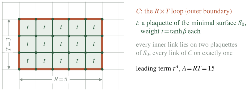
Figure 1. The tiled Wilson loop: the link sums leave the links of $C$ unpaired unless every plaquette inside $C$ is used once, so the leading term is $t^A$ with $A=RT$.

4.2 Leading order and the first correction [Controlled to $O(t^4)$ in $t=\tanh \beta$.]

For a planar $R\times T$ rectangle let $S_0$ be the flat surface of $A=RT$ plaquettes. Every surface with $\partial S=C$ is $S=S_0\oplus Z$ with $Z$ closed ($\oplus$ is addition mod 2, the symmetric difference of plaquette sets), and

$$|S_0\oplus Z|=A+|Z|-2|S_0\cap Z|.$$

On the infinite lattice every closed surface bounds a finite set of cubes; the smallest is the boundary of a single cube, $|\partial c|=6$, and a cube shares at most one plaquette with the flat $S_0$, because its two faces parallel to $S_0$ lie in different planes. The terms through relative order $t^4$ are therefore:

surface	$|S|$	number	weight relative to $t^A$
$S_0$	$A$	1	1
$S_0\oplus \partial c$, with $c$ having a face in $S_0$	$A+4$	$2(d-2)A$	$t^4$
all others	$\ge A+6$		$O(t^6)$

The count $2(d-2)A$ holds because a plaquette in the $(\mu ,\nu )$ plane is a face of one cube in each of the $2(d-2)$ transverse half-directions; Figure 2 shows one such decoration. The denominator is $1+N_c{t}^6+\dots$, with no $t^4$ term. Thus $⟨W(C)⟩=t^A[1+2(d-2)A{t}^4+O(t^6)]$, and taking the logarithm,

$$\ln ⟨W(C)⟩=A\ln t+2(d-2)A{t}^4+O(t^6),\boxed{\sigma =-\ln \tanh \beta -2(d-2){\tanh }^4\beta +O({\tanh }^6\beta ),}$$

where the string tension σ is defined by $⟨W(C)⟩\sim e^{-\sigma A}$ for large loops. The $t^4$ term has no perimeter part, since the plaquettes along $C$ carry their $2(d-2)$ cubes like the interior ones. The perimeter dependence first appears at relative order $t^6$, where cubes that share only a link with $S_0$ cancel against the denominator and bricks of two cubes resting on $S_0$ enter (Problem 3).

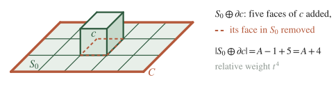
Figure 2. A decorated surface: the face of the cube $c$ that lay in $S_0$ cancels mod 2 and its other five faces are added, $|S_0\oplus \partial c|=A-1+5=A+4$; it is the lowest transverse fluctuation of the flux sheet.

Four checks. (i) Wegner’s eq. (3.34) for $n=2$ reads $[t+2(d-2)t^5+\dots {]}^A$, the same result. (ii) For the $1\times 1$ loop, $⟨W(\partial P)⟩=⟨{\sigma }_P⟩=N_P^{-1}{\partial }_{\beta }\ln Z$, and $\ln Z=N_{\ell }\ln 2+N_P\ln \cosh \beta +N_c{t}^6+O(t^{10})$ gives $⟨{\sigma }_P⟩=t+6(N_c/N_P)t^5+O(t^7)=t+2(d-2)t^5+O(t^7)$, since $N_c/N_P=(d-2)/3$; this is the loop formula at $A=1$. (iii) Complete enumeration of all subsets of cubes in open boxes gives the $t^4$ coefficient of $\ln (⟨W⟩/t^A)$ exactly $2(d-2)A$ for the $1\times 1$, $1\times 2$, $1\times 3$, $2\times 2$ and $2\times 3$ loops (in $d=4$ with the cubes resting on $S_0$, and a full box for $1\times 1$). (iv) At $d=2$ the correction vanishes, as it must by §6.

Physical picture. A rectangular $R\times T$ loop is the worldline of a static pair of ${\mathbb{Z}}_2$ charges at separation $R$ for a time $T$, and $V(R)=-{\lim }_{T\to \infty }{T}^{-1}\ln ⟨W(R\times T)⟩$ is their potential (Week 7 obtains $V(R)$ as the energy of the static pair in the Hamiltonian formulation). At strong coupling the electric flux of the pair fills the minimal sheet, $V(R)=\sigma R$ grows linearly, and the charges are confined (confinement). The decorations are the sheet’s first transverse fluctuations; as β grows they proliferate and the sheet roughens, which Week 6 takes up. The strong-coupling expansion converges for small β, so the area law is a theorem there [Stated — refs: Osterwalder–Seiler 1978]. Confinement at strong coupling holds for every gauge group; the question of the week is whether it survives at weak coupling.

5. Weak coupling: the perimeter law [Controlled to leading order in $e^{-4\beta }$.]

At large β we expand around the configurations with every ${\sigma }_P=+1$. A gauge transformation changes no ${\sigma }_P$, so we label each gauge class by one representative (Kogut’s “representative configurations”, §V.D); the orbit size $2^{N_s-1}$ is common to numerator and denominator and cancels. Starting from $\sigma \equiv 1$, reverse one link $\ell$. The $2(d-1)$ plaquettes that contain $\ell$ become frustrated, each at a cost $2\beta$, so the configuration has relative weight

$$w\equiv e^{-4(d-1)\beta }.$$

In $d=3$ the four frustrated plaquettes are pierced by a small closed dual loop around $\ell$ (Figure 3): a reversed link is the smallest closed vison loop, and it links $C$ exactly when $\ell \in C$, where $W(C)=-1$. To first order in $w$,

$$⟨W(C)⟩=\frac{1+(N_{\ell }-|C|)w-|C|w+O(w^2)}{1+N_{\ell }w+O(w^2)}=1-2|C|w+O(w^2),$$

where $|C|$ is the number of links of $C$. Reversals of different links contribute independent factors unless the links share a plaquette, so they exponentiate as a dilute gas,

$$⟨W(C)⟩\simeq \prod _{\ell \in C}\frac{1-w}{1+w}=\exp (-2w|C|+O(w^3|C|)),$$

and the pairs of reversed links that share a plaquette, of weight $w^2{e}^{4\beta }$ (the common plaquette is reversed twice, and therefore not frustrated), correct the exponent at relative order $w{e}^{4\beta }=e^{-4(d-2)\beta }$. Therefore

$$\boxed{⟨W(C)⟩\simeq e^{-\mu |C|},\mu =2e^{-4(d-1)\beta }[1+O(e^{-4(d-2)\beta })](d\ge 3).}$$

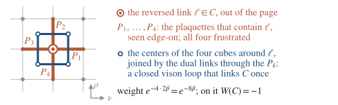
Figure 3. Weak coupling in $d=3$: a reversed link of $C$ frustrates the four plaquettes that contain it; the frustration is a unit vison loop that links $C$ once and reverses $W(C)$, which gives $\mu =2e^{-8\beta }$.

Three checks. (i) The partition function alone: $\ln Z=\beta N_P+\ln 2^{N_s-1}+N_{\ell }w+O(w^2)$ gives $⟨{\sigma }_P⟩=1-(N_{\ell }/N_P)4(d-1)w=1-8w$, since $N_{\ell }/N_P=2/(d-1)$, and the loop formula with $|C|=4$ gives the same $1-2\cdot 4\cdot w$. (ii) Kogut’s eq. (5.32) gives the leading term $2\exp [-4(d-1)\beta ]$. (iii) In $d=3$ the next order is explicit for the $1\times 1$ loop: 44 vison loops of length 6 link it (36 pairs of reversed links that share a plaquette and 8 corner triples), so on the infinite lattice $(1-⟨W⟩)/(|C|w)=2+22e^{-4\beta }+\dots$, that is $2.000999$ at $\beta =2.5$. We computed $⟨W⟩$ exactly through the dual Ising model of §7, with a transfer matrix and all eight boundary sectors (F6), on $3\times 3\times L$ tori with $L\ge 4$ and the loop in the $3\times 3$ plane, and obtained this value; the deviation from 2 falls by $e^{-2}$ per $\Delta \beta =0.5$, the $e^{-4\beta }$ of the correction term. (On the $3\times 3\times 3$ torus, or with the loop in a plane that contains the long direction, pairs of winding vison loops add a finite-size shift of order $10^{-4}$.)

There is no area term at weak coupling. A vison loop reverses $W(C)$ only if it links $C$, and a loop that links $C$ through the interior of $S_0$ far from $C$ must close around $C$, so its length and its cost $e^{-2\beta \cdot \text{length}}$ grow with the distance to $C$. Summed over positions these loops give contributions proportional to $|C|$: they renormalize μ. The pair potential then tends to the constant $2\mu$, twice the self-energy of an isolated charge, and the charges are free. The low-temperature expansion converges at large β in $d\ge 3$ (Kogut §V.D), so the deconfined phase exists and differs from the confined phase of §4. In $d=2$ the argument fails at its first step: reversing a whole row of links frustrates only the two plaquettes at its ends (Kogut, Fig. 26), strings of reversals of any length cost a finite amount, so every order of the expansion is proportional to the area and none produces a perimeter law; the sum is $⟨W⟩=((1-u)/(1+u){)}^A=(\tanh \beta {)}^A$ with $u=e^{-2\beta }$, and §6 shows that the loop obeys an area law at every β.

Physical picture. The two expansions give two pictures of the vacuum. At weak coupling it is a dilute gas of small closed vison loops, each dressing the charges locally, and electric flux spreads freely. At strong coupling magnetic flux is so cheap that vison loops of every size are present, and an electric flux sheet is the only way two charges can communicate. Confinement is the proliferation of the magnetic defects, the ${\mathbb{Z}}_2$ prototype of the defect-condensation mechanism of the group’s Julia–Toulouse program (julia-toulouse-mechanism, condensation-defects). In $d=3$ §7 makes the statement exact: proliferated visons are the ordered phase of an Ising model.

6. Two dimensions: confinement at every coupling [Computed.]

Take a finite rectangle of plaquettes with open boundary conditions. It is contractible, so $N_s-N_{\ell }+N_P=1$, and a flat configuration (every ${\sigma }_P=+1$) is pure gauge, $\sigma =dϵ$. The map $\sigma \mapsto ({\sigma }_P{)}_P$ therefore has $2^{N_s-1}$ preimages for each point of its image, and the image has $2^{N_{\ell }}/2^{N_s-1}=2^{N_P}$ points: every assignment of plaquette signs occurs. With no cubes there is no Bianchi identity, and the plaquette variables are independent:

$$Z=2^{N_s-1}(2\cosh \beta {)}^{N_P}.$$

For a loop $C$ enclosing the set $S$ of $A$ plaquettes, $W(C)={\prod }_{P\in S}{\sigma }_P$ by Stokes, and independence gives

$$\boxed{⟨W(C)⟩=(\tanh \beta {)}^A\text{exactly, at every }\beta .}$$

This is a genuine area law with $\sigma =-\ln \tanh \beta$ at every coupling: the 2d theory confines everywhere, has no transition, and every correction to the strong-coupling tension vanishes, as the factor $2(d-2)$ of §4.2 already showed at first order.

The same result follows in a complete gauge. Fix $\sigma =1$ on all horizontal links and on the vertical links of the first column, a comb-shaped maximal tree. Each plaquette then reads ${\sigma }_P={\sigma }_v(x,y){\sigma }_v(x+1,y)$, the product of its two vertical links, so the vertical links of each row form an open Ising chain of coupling β with its first spin fixed, and different rows decouple. A rectangular $R\times T$ loop becomes ${\prod }_{\mathrm{rows}}{\sigma }_v(x_0,y){\sigma }_v(x_0+R,y)$, and the chain correlator $⟨s_0{s}_R⟩=t^R$ gives $t^{RT}$. The 2d gauge theory is a stack of decoupled Ising chains, and Ising chains never order.

On the torus two things change. Each link lies on exactly two plaquettes, so ${\prod }_P{\sigma }_P=1$ identically, and there are flat configurations that are not pure gauge, classified by $H^1(T^2,{\mathbb{Z}}_2)={\mathbb{Z}}_2^2$, so that each allowed plaquette configuration has $4\cdot 2^{N_s-1}$ preimages. With the projector $\frac{1}{2}(1+{\prod }_P{\sigma }_P)$,

$$Z=2^{N_s}[(2\cosh \beta {)}^{N_P}+(2\sinh \beta {)}^{N_P}],⟨W(C)⟩=\frac{t^A+t^{N_P-A}}{1+t^{N_P}}$$

for a contractible $C$, which tends to $t^A$ at fixed $A$ as $N_P\to \infty$; complete enumeration on the $3\times 3$ torus reproduces this formula to twelve digits for $A=1,2,4$ at $\beta =0.3$ and $1$. In $1+1$ dimensions the electric flux of a static charge cannot spread, and its energy grows with its length at every coupling.

7. Three dimensions: the duality to the Ising model

7.1 Surfaces and walls [Computed.]

In $d=3$ the dual lattice of Week 2 (conventions §2) pairs dual sites with cubes, dual links with plaquettes, dual plaquettes with links and dual cubes with sites. Place Ising spins $s\in C^0({\Lambda }^{\ast },{\mathbb{Z}}_2)$ on the dual sites, with coupling $K^{\ast }$ on the dual links $b$:

$$Z_I(K^{\ast })=\sum _s\exp (K^{\ast }\sum _b(ds)(b)),(ds)(b)=s_{\tilde{x}}{s}_{\tilde{y}}\text{ for }b=⟨\tilde{x}\tilde{y}⟩.$$

Expand at low temperature, as in Week 4 §3.2 with one more dimension. Writing $s=(-1{)}^{\phi }$, a bond is broken when $(d\phi )(b)=1$. The broken bonds are dual to a set of plaquettes $W=\star d\phi$, and the transport rule “coboundary on ${\Lambda }^{\ast }$ ↔ boundary on Λ” of Week 2 §5.2 gives $W=\partial (\star \phi )$, where $\star \phi$ is the set of cubes whose spin is reversed. A domain wall is thus a closed surface of Λ that bounds a set of cubes, and each broken bond lowers the exponent by $2K^{\ast }$. For a box with free boundary conditions on the gauge side, these walls are exactly the domain walls of the Ising model on the cubes of the box with the spins outside the box fixed to $+1$, and

$$Z_I^{+}(K^{\ast })=e^{K^{\ast }{N}_P}\sum _K{e}^{-2K^{\ast }|\partial K|},$$

where $K$ runs over sets of cubes and there is one Ising bond per plaquette. The gauge sum of §4.1 runs over the same surfaces, since every closed surface in a box bounds a unique set of cubes, with weight $t^{|S|}$ in place of $e^{-2K^{\ast }|W|}$ (Figure 4). The weights match term by term exactly when

$$\boxed{\tanh \beta =e^{-2K^{\ast }}⟺\sinh 2\beta \sinh 2K^{\ast }=1⟺\tanh K^{\ast }=e^{-2\beta },}$$

where the equivalences are the algebra of Week 4 §3.3. With $\cosh \beta e^{-K^{\ast }}=(\frac{1}{2}\sinh 2\beta {)}^{1/2}=(2\sinh 2K^{\ast }{)}^{-1/2}$ the prefactors combine to

$$Z_g(\beta )=2^{N_{\ell }}(2\sinh 2K^{\ast }{)}^{-N_P/2}{Z}_I^{+}(K^{\ast }).$$

The prefactor is analytic at every $\beta >0$, so the free energies of the two models differ by an analytic function and are singular at the same point. Since $\tanh \beta$ increases with β while $e^{-2K^{\ast }}$ decreases with $K^{\ast }$, strong coupling is low temperature: the confined phase is the ordered Ising phase and the deconfined phase is the disordered one (conventions §4). The 3d Ising critical coupling $K_c^{\ast }=0.221654626(5)$ [Stated — refs: Ferrenberg, Xu, Landau, Phys. Rev. E 97 (2018) 043301] then locates the gauge transition:

$$\boxed{{\beta }_c=\mathrm{artanh}\left(e^{-2K_c^{\ast }}\right)=\mathrm{0.7614133.}}$$

On the torus the same identity holds with a sum over the eight boundary sectors of the Ising model (F6).

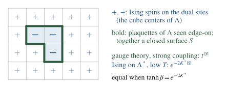
Figure 4. The 3d duality in one picture (a cross-section): a closed surface of plaquettes, weighted $t^{|S|}$ in the strong-coupling expansion of the gauge theory, is the domain wall around a cluster of reversed dual spins, weighted $e^{-2K^{\ast }|S|}$ in the low-temperature expansion of the Ising model on ${\Lambda }^{\ast }$; the weights agree when $\tanh \beta =e^{-2K^{\ast }}$.

7.2 The Wilson loop is a pinned interface [Computed; the identification of the tension Sketched.]

Choose a surface Σ with $\partial \Sigma =C$ and reverse the Ising couplings, $K^{\ast }\to -K^{\ast }$, on the bonds ${\Sigma }^{\ast }$ dual to its plaquettes. In a configuration whose broken bonds are dual to $W=\partial K$, the bonds that now lower the exponent are those dual to $\Sigma \oplus W$, so the steps of §7.1 give $Z_I^{+}[K^{\ast }\to -K^{\ast }\text{ on }{\Sigma }^{\ast }]=e^{K^{\ast }{N}_P}{\sum }_K{e}^{-2K^{\ast }|\Sigma \oplus \partial K|}$, and the surfaces $\Sigma \oplus \partial K$ are exactly those with boundary $C$. Comparing with the numerator of §4.1,

$$\boxed{⟨W(C){⟩}_{\beta }=\frac{Z_I[K^{\ast }\to -K^{\ast }\text{on}{\Sigma }^{\ast }]}{Z_I(K^{\ast })},}$$

independent of the choice of Σ, since reversing the couplings on the bonds dual to $\partial K$ is undone by $s\to -s$ on $K$. In the ordered phase the reversed bonds force a domain wall that ends on $C$. For a large planar loop its free energy per unit area is the interface tension $\tau (K^{\ast })$ of the Ising model, so ${\sigma }_{\mathrm{gauge}}(\beta )={\tau }_{\mathrm{Ising}}(K^{\ast })$: the string tension of the 3d ${\mathbb{Z}}_2$ gauge theory is the interface tension of the 3d Ising model [Sketched: the passage from the pinned wall to τ for large loops is the definition of the interface tension, which we do not prove here]. In the disordered phase no wall survives at large scales and the reversed bonds cost only near $C$, a perimeter law. The string tension therefore vanishes at ${\beta }_c$ together with the interface tension, and Problem 2 recovers $\sigma =-\ln t-2t^4$ from the interface side.

7.3 The vison is the dual Ising spin [Computed.]

Choose a dual path $\tilde{\gamma }$ from $\tilde{x}$ to $\tilde{y}$ and reverse the coupling, $\beta \to -\beta$, on the plaquettes it pierces (the plaquettes dual to its dual links), a set we call ${\tilde{\gamma }}^{\ast }$. Define

$$⟨\mu (\tilde{x})\mu (\tilde{y}){⟩}_{\beta }\equiv \frac{Z_g[\beta \to -\beta \text{on}{\tilde{\gamma }}^{\ast }]}{Z_g}.$$

String independence. Two paths with the same endpoints differ by a closed dual loop $\tilde{\ell }=\tilde{\gamma }\oplus {\tilde{\gamma }}^{\prime }$, which on the infinite lattice bounds a dual surface $\tilde{\Sigma }$. Let $\lambda \in C^1(\Lambda ,{\mathbb{Z}}_2)$ be $-1$ on the links dual to the dual plaquettes of $\tilde{\Sigma }$. A plaquette $P$ has $(d\lambda {)}_P=-1$ when an odd number of its four links is in λ, and its four links are dual to the four dual plaquettes that contain the dual link $P^{\ast }$; so $(d\lambda {)}_P=-1$ exactly when $P^{\ast }\in \partial \tilde{\Sigma }=\tilde{\ell }$. The change of variables $\sigma \to \sigma \lambda$ therefore carries the reversal on ${\tilde{\gamma }}^{\ast }$ to the reversal on ${\tilde{\gamma }}^{\prime \ast }$: only the endpoints are physical, as for the Kadanoff–Ceva seam of Week 4 §4.1.

Identification. In the surface expansion the reversal changes $t\to -t$ on ${\tilde{\gamma }}^{\ast }$, so each closed surface $S$ acquires the sign $(-1{)}^{|S\cap {\tilde{\gamma }}^{\ast }|}$. Read $S$ as a domain wall: $|S\cap {\tilde{\gamma }}^{\ast }|$ counts the broken bonds along $\tilde{\gamma }$, and $(-1{)}^{|S\cap {\tilde{\gamma }}^{\ast }|}={\prod }_{b\in \tilde{\gamma }}(ds)(b)=s_{\tilde{x}}{s}_{\tilde{y}}$. Therefore

$$\boxed{⟨\mu (\tilde{x})\mu (\tilde{y}){⟩}_{\beta }=⟨s_{\tilde{x}}{s}_{\tilde{y}}{⟩}_{K^{\ast }},}$$

which complete enumeration confirms on the $2^3$ torus at four couplings (with the sector sum of F6). The dual Ising spin is the endpoint of a string of flipped plaquettes: the vison (Figure 5a).

The two phases at leading order. At strong coupling the smallest closed surfaces are cube boundaries, and $|\partial c\cap {\tilde{\gamma }}^{\ast }|$ is the number of dual links of $\tilde{\gamma }$ at the dual site $c^{\ast }$, odd only for the two endpoint cubes. Thus, for well-separated endpoints,

$$⟨\mu \mu ⟩=\frac{1+(N_c-2)t^6-2t^6+\dots }{1+N_c{t}^6+\dots }=1-4t^6+O(t^{10}),$$

the square of the dual magnetization $m^{\ast }=1-2e^{-12K^{\ast }}+\dots$: in the confined phase the visons are condensed. At weak coupling we use the frustration expansion of §5. The Bianchi identity makes the frustrated plaquettes of $Z_g$ a set of closed dual loops, and reversing the coupling on ${\tilde{\gamma }}^{\ast }$ moves its violation to the endpoints, so the frustrated plaquettes now form dual paths from $\tilde{x}$ to $\tilde{y}$ (plus closed loops), at a cost $e^{-2\beta }$ per plaquette. Along a lattice axis,

$$⟨\mu (\tilde{x})\mu (\tilde{y})⟩\simeq e^{-2\beta r}[1+2r(r+1)e^{-4\beta }+\dots ],r=|\tilde{x}-\tilde{y}|,$$

the Ising high-temperature correlator $(\tanh K^{\ast }{)}^r$ with its first correction. The correction counts the paths with one transverse excursion, four transverse directions times $r(r+1)/2$ placements, each two plaquettes longer; since it grows with $r$, it is a shift of the mass, which we read off from the pole of the path sum: with $u=e^{-2\beta }$, $1=2u(\cosh \kappa +2)$ gives $e^{-\kappa }=u(1+4u+\dots )$. In the deconfined phase the visons are therefore gapped particles of mass $m=2\beta -4e^{-2\beta }+O(e^{-4\beta })$. In the form-degree table of conventions §6, μ is local in $d=3$, like the ‘t Hooft operators of dimension $d-3=0$ and the monopole operator $e^{i\sigma }$ of compact QED₃ (Week 9). In gauge variables it carries an unobservable string, like the Kadanoff–Ceva μ; in Ising variables it is the genuine spin.

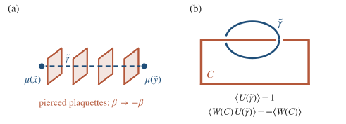
Figure 5. (a) The vison pair $\mu (\tilde{x})\mu (\tilde{y})$: the string is invisible and only its endpoints are physical. (b) A closed dual string $\tilde{\gamma }$ linking a Wilson loop: $⟨U(\tilde{\gamma })⟩=1$ and $⟨W(C)U(\tilde{\gamma })⟩=-⟨W(C)⟩$ (§8.1).

7.4 The Hamiltonian cross-check [Computed.]

The $2+1$ Hamiltonian of conventions §4 is $H=-\Gamma {\sum }_{\ell }{\sigma }_{\ell }^x-K{\sum }_P{B}_P$, with $B_P={\prod }_{\ell \in \partial P}{\sigma }_{\ell }^z$, ${\sigma }_{\ell }^z$ the link variable, ${\sigma }_{\ell }^x=(-1{)}^{E_{\ell }}$ the electric field, and physical states obeying Gauss’s law ${\prod }_{\ell \ni v}{\sigma }_{\ell }^x=1$. On the dual sites (the plaquettes of the spatial lattice) define

$${\mu }_P^x=B_P,{\mu }_P^z=\prod _{\ell \text{crossed by a dual path from }P\text{ to infinity}}{\sigma }_{\ell }^x,$$

so that ${\mu }_P^z{\mu }_{P^{\prime }}^z={\sigma }_{\ell }^x$ for the two plaquettes $P,P^{\prime }$ that share ℓ. Three checks. (i) The Pauli algebra: $B_P$ anticommutes with ${\sigma }_{\ell }^x$ exactly when $\ell \in \partial P$, and ${\mu }_P^x$ anticommutes with ${\mu }_Q^z{\mu }_{Q^{\prime }}^z$ exactly when $P\in \{Q,Q^{\prime }\}$, the same condition. (ii) Gauss’s law: ${\prod }_{\ell \ni v}{\sigma }_{\ell }^x$ becomes a product of ${\mu }^z{\mu }^z$ around the four plaquettes at $v$, in which each ${\mu }_P^z$ appears twice, so it equals 1 and the dual variables describe exactly the physical sector. (iii) The Hamiltonian becomes

$$H=-\Gamma \sum _{⟨P{P}^{\prime }⟩}{\mu }_P^z{\mu }_{P^{\prime }}^z-K\sum _P{\mu }_P^x,$$

the transverse-field Ising model on the dual lattice. Strong coupling, $\Gamma \gg K$, is its ferromagnetic phase, with $⟨{\mu }^z⟩\ne 0$: the confined phase is again the ordered Ising phase, and the order parameter is the string of electric-field operators, Kogut’s “kink” operator, whose condensation at strong coupling is his eq. (5.69). The derivation of $H$ from the transfer matrix, with Γ and K expressed through the anisotropic couplings ${\beta }_t$ and ${\beta }_s$, is Week 7.

8. The electric 1-form symmetry and the ‘t Hooft operators

8.1 Closed sheets are symmetry operators [Computed.]

Consider a closed dual $(d-2)$-chain $\tilde{\Sigma }$ that bounds a dual $(d-1)$-chain $\tilde{V}$, $\tilde{\Sigma }=\partial \tilde{V}$; on the infinite lattice every closed $\tilde{\Sigma }$ does. In $d$ dimensions a plaquette is dual to a $(d-2)$-cell, so let $F$ be the set of plaquettes dual to the cells of $\tilde{\Sigma }$, and let $\lambda \in C^1(\Lambda ,{\mathbb{Z}}_2)$ be $-1$ on the links dual to the cells of $\tilde{V}$. The argument of §7.3 in any dimension gives $d\lambda =-1$ exactly on $F$. Define $U(\tilde{\Sigma })$ by reversing the coupling on $F$, $⟨U(\tilde{\Sigma })⟩=Z[\beta \to -\beta \text{ on }F]/Z$, and similarly with $W(C)$ inserted. Substitute $\sigma ={\sigma }^{\prime }\lambda$. Then ${\sigma }_P={\sigma }_P^{\prime }(d\lambda {)}_P$, so the reversed plaquette term $(-1{)}^{[P\in F]}{\sigma }_P$ equals ${\sigma }_P^{\prime }$ on every plaquette, while

$$W(C;\sigma )=W(C;{\sigma }^{\prime })\prod _{\ell \in C}{\lambda }_{\ell }=W(C;{\sigma }^{\prime })(-1{)}^{\#(C\cap \tilde{V})},$$

where $\#(C\cap \tilde{V})$, the number of links of $C$ dual to cells of $\tilde{V}$, is the intersection number of $C$ with a chain bounded by $\tilde{\Sigma }$, that is, the linking number $\mathrm{Link}(C,\tilde{\Sigma })$ mod 2. Therefore, at every β and in every phase,

$$\boxed{⟨U(\tilde{\Sigma })⟩=1,⟨W(C)U(\tilde{\Sigma })⟩=(-1{)}^{\mathrm{Link}(C,\tilde{\Sigma })}⟨W(C)⟩.}$$

In $d=3$, $\tilde{\Sigma }$ is a closed dual loop and $F$ is the set of plaquettes it pierces (Figure 5b); in $d=4$, $\tilde{\Sigma }$ is a closed dual surface. The operator $U(\tilde{\Sigma })$ is invisible by itself, can be deformed at will, and detects Wilson loops by linking: it is the symmetry operator of the electric ${\mathbb{Z}}_2$ 1-form symmetry (higher-form-symmetries). The transformation it implements is $\sigma \to \sigma \lambda$ with λ closed, the lattice form of $a\to a+\lambda$ with $d\lambda =0$; exact λ are gauge transformations, and the classes in $H^1(\Lambda ,{\mathbb{Z}}_2)$ act nontrivially on a torus. Form-degree check against conventions §6: a 1-form symmetry in $d$ dimensions has operators on closed $(d-1-1)$-dimensional manifolds, dual loops in $d=3$ and dual surfaces in $d=4$, and its charged objects are Wilson lines. In the Hamiltonian slice, $U$ is the product of ${\sigma }_{\ell }^x$ over the links crossing a closed dual $(d-2)$-surface of space, the parity of the electric flux through it; it commutes with $H$, and Gauss’s law lets it be deformed.

The charged loop is the order parameter of this symmetry. By the criterion of conventions §6, an area law means the symmetry is unbroken and a perimeter law (after the counterterm of F3) means it is spontaneously broken. Thus the deconfined phases of §§5 and 7 break ${\mathbb{Z}}_2^{(1)}$ spontaneously, the confined phase preserves it, and in $d=2$ it is never broken, which §6 reduced to the fact that Ising chains never order.

8.2 Open sheets: visons in $d=3$, ‘t Hooft loops in $d=4$ [Computed at leading order.]

When the reversed set $F$ is dual to a $(d-2)$-chain $\tilde{\Sigma }$ with a boundary, the reversal cannot be removed: at each cube $c$ dual to a $(d-3)$-cell of $\partial \tilde{\Sigma }$ the effective field strength violates the Bianchi identity, ${\prod }_{P\in \partial c}(-1{)}^{[P\in F]}{\sigma }_P=-1$. The boundary $\partial \tilde{\Sigma }$ is the worldvolume of a ${\mathbb{Z}}_2$ magnetic source and $\tilde{\Sigma }$ is its Dirac sheet, movable by the change of variables of §8.1. These are the ‘t Hooft operators, of dimension $d-3$ (conventions §6):

• in $d=3$, $\partial \tilde{\Sigma }=\{\tilde{x},\tilde{y}\}$: the vison pair $\mu (\tilde{x})\mu (\tilde{y})$ of §7.3, local operators on a Dirac string;
• in $d=4$, $\partial \tilde{\Sigma }=\tilde{C}$ is a closed dual loop: the ‘t Hooft loop $\tilde{W}(\tilde{C})$ reverses β on the plaquettes dual to the 2-cells of a dual surface $\tilde{S}$ with $\partial \tilde{S}=\tilde{C}$ (in $d=4$ plaquettes and dual 2-cells are dual to each other).

With a Wilson loop present, moving the sheet across $C$ multiplies $⟨W(C)\cdots ⟩$ by $-1$ whenever $C$ crosses the swept region an odd number of times; this is the gauge-theory form of the σ–μ crossing sign of Week 4 §4.3.

The four-dimensional ‘t Hooft loop at leading order in its two phases. Strong coupling. In the surface expansion each closed surface acquires the sign $(-1{)}^{|S\cap F|}$. A face $P$ of a cube $c$ corresponds to a dual 2-cell $P^{\ast }$ that has the dual link $c^{\ast }$ in its boundary, so $|\partial c\cap F|$ counts the 2-cells of $\tilde{S}$ at $c^{\ast }$, which is odd exactly when $c^{\ast }\in \partial \tilde{S}=\tilde{C}$: one cube per dual link of $\tilde{C}$. Therefore

$$⟨\tilde{W}(\tilde{C})⟩=\frac{1+(N_c-|\tilde{C}|)t^6-|\tilde{C}|t^6+\dots }{1+N_c{t}^6+\dots }=1-2|\tilde{C}|t^6+\cdots \simeq e^{-2t^6|\tilde{C}|},$$

a perimeter law with $\tilde{\mu }=2t^6$ at leading order. Weak coupling. In the frustration expansion the Bianchi identity makes the frustrated plaquettes closed dual surfaces, and the reversed sheet moves the violation to $\tilde{C}$: the frustrated plaquettes form a dual surface bounded by $\tilde{C}$, at $e^{-2\beta }$ per plaquette, so the minimal one dominates and

$$⟨\tilde{W}(\tilde{C})⟩\simeq e^{-2\beta A(\tilde{C})},$$

an area law with $\tilde{\sigma }=2\beta$ at leading order. In $d=4$ the two loops exchange roles: at strong coupling $W$ has an area law and $\tilde{W}$ a perimeter law, at weak coupling the reverse, as in ‘t Hooft’s classification of massive phases [Stated — refs: ‘t Hooft, Nucl. Phys. B 138 (1978) 1].

8.3 Self-duality in $d=4$ and the ‘t Hooft algebra [Computed.]

In $d=4$ the frustrated plaquettes of the weak-coupling expansion are dual to 2-cells of ${\Lambda }^{\ast }$, and the Bianchi identity, an even number of frustrated faces on every cube, that is, on every dual link, says that they form closed dual surfaces with weight $e^{-2\beta }$ per cell. The strong-coupling expansion of the same theory on ${\Lambda }^{\ast }$ at a coupling ${\beta }^{\ast }$ is a sum over closed surfaces with weight $(\tanh {\beta }^{\ast }{)}^{|S|}$. The two agree when $\tanh {\beta }^{\ast }=e^{-2\beta }$, which is

$$\sinh 2\beta \sinh 2{\beta }^{\ast }=1,{\beta }_{\mathrm{sd}}=\frac{1}{2}\ln (1+\sqrt{2})=0.4406868$$

(conventions §4), so the free energies at β and ${\beta }^{\ast }$ differ by an analytic function (with the sector bookkeeping of F6 on a torus). Operator by operator, the frustration expansion of $\tilde{W}(\tilde{C})$ at β, dual surfaces bounded by $\tilde{C}$, is the surface expansion of $W(\tilde{C})$ at ${\beta }^{\ast }$:

$$⟨\tilde{W}(\tilde{C}){⟩}_{\beta }=⟨W(\tilde{C}){⟩}_{{\beta }^{\ast }}.$$

This checks the computations of §§5 and 8.2 against each other: the strong-coupling ‘t Hooft coefficient $\tilde{\mu }(\beta )=2t^6$ equals the weak-coupling Wilson coefficient $\mu ({\beta }^{\ast })=2e^{-12{\beta }^{\ast }}$ of §5 at $d=4$, since $e^{-2{\beta }^{\ast }}=\tanh \beta$. If the model has a single transition, it sits at ${\beta }_{\mathrm{sd}}$; it is first order there [Stated — refs: Kogut §V.E, which reviews the free-energy expansions and the Monte Carlo evidence]. As in Week 4, the duality locates a singularity, and its existence and order are separate input.

The ‘t Hooft algebra follows in the Hamiltonian slice of the 4d theory, which has three spatial dimensions. Take $W(C)={\prod }_{\ell \in C}{\sigma }_{\ell }^z$ on a spatial loop and $\tilde{W}(\tilde{C})={\prod }_{\ell \text{pierced by}\tilde{S}}{\sigma }_{\ell }^x$, with $\tilde{S}$ a spatial dual surface bounded by the dual loop $\tilde{C}$. The operator $\tilde{W}$ reverses ${\sigma }^z$ on the links pierced by $\tilde{S}$, which frustrates exactly the plaquettes dual to the dual links of $\tilde{C}$: it creates a closed loop of magnetic flux along $\tilde{C}$. Since ${\sigma }_{\ell }^z$ and ${\sigma }_{\ell }^x$ anticommute on each link of $C$ pierced by $\tilde{S}$ and commute otherwise,

$$W(C)\tilde{W}(\tilde{C})=(-1{)}^{\#(C\cap \tilde{S})}\tilde{W}(\tilde{C})W(C)=(-1{)}^{\mathrm{Link}(C,\tilde{C})}\tilde{W}(\tilde{C})W(C),$$

‘t Hooft’s commutation relation. In $d=3$ the spatial closed string $U(\tilde{\gamma })$ anticommutes with $W(C)$ when the two curves cross an odd number of times, which on a spatial torus happens for the noncontractible pairs: the algebra behind the four ground states of Problem 5⋆.

Physical picture. Electric and magnetic probes are mutually non-local, so they cannot condense together: this is the exclusivity of order and disorder operators of Week 4 §4.2, now for loops. In the confined phase magnetic flux is condensed (visons in $d=3$, where $⟨\mu \mu ⟩$ tends to a constant; monopole loops in $d=4$, where $\tilde{W}$ has a perimeter law), and an electric flux line has nowhere to go but a sheet of tension σ. In the deconfined phase electric flux is free, magnetic flux costs $2\beta$ per plaquette, and the roles are exchanged. This is the ${\mathbb{Z}}_2$ prototype of the dual-superconductor picture of Week 11, exact here. In the language of §8.1 it says that the deconfined phase breaks ${\mathbb{Z}}_2^{(1)}$ while its dual Ising model preserves ${\mathbb{Z}}_2^{(0)}$, and conversely in the confined phase: the duality exchanges broken and unbroken symmetries, as gauging does in general (conventions §6; Semester II Week 4) [Stated — forward reference].

9. Phase structure by dimension

Figure 6 and the table collect the results of §§4–8.

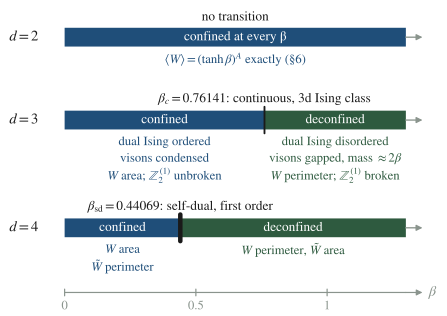
Figure 6. Phase structure of the ${\mathbb{Z}}_2$ gauge theory by dimension: no transition in $d=2$, a continuous transition in the 3d Ising class at ${\beta }_c=0.76141$ in $d=3$, a first-order transition at the self-dual point ${\beta }_{\mathrm{sd}}=0.44069$ in $d=4$.

$d$	exact tool	transition	confined phase	deconfined phase
2	independent plaquettes (§6)	none	every β; $\sigma =-\ln \tanh \beta$	none
3	$\tanh \beta =e^{-2K^{\ast }}$ to 3d Ising (§7)	${\beta }_c=0.76141$, continuous	$\beta <{\beta }_c$: Ising ordered, visons condensed	$\beta >{\beta }_c$: Ising disordered, ${\mathbb{Z}}_2$ topological order
4	$\sinh 2\beta \sinh 2{\beta }^{\ast }=1$ (§8.3)	${\beta }_{\mathrm{sd}}=0.44069$, first order	$\beta <{\beta }_{\mathrm{sd}}$: $W$ area, $\tilde{W}$ perimeter	$\beta >{\beta }_{\mathrm{sd}}$: $W$ perimeter, $\tilde{W}$ area

The deconfined phase of the 3d model is the ${\mathbb{Z}}_2$ topological-order of the toric-code (F5; Semester II Week 8).

10. Subtleties and fine print

F1 — Why the bound is uniform in the volume. The proof of §3.1 compared σ with $g_x\sigma$, whose weights differ by at most $e^{4d|h|}$, because a local transformation touches $2d$ source terms whatever the size of the lattice. The two limits then commute: ${\lim }_{h\to 0}{\lim }_{V\to \infty }⟨{\sigma }_{\ell }⟩={\lim }_{V\to \infty }{\lim }_{h\to 0}⟨{\sigma }_{\ell }⟩=0$. For the Ising magnetization the only transformation available is global, the weights differ by up to $e^{2N|h|}$, and the order of the limits decides the answer: the thermodynamic limit at fixed $h>0$ selects a state, and the limit $h\to 0^{+}$ taken afterwards leaves $m(\beta )\ne 0$ below $T_c$. Spontaneous symmetry breaking lives in the non-commutativity of these two limits, and Elitzur’s bound removes it for local symmetries.

F2 — Gauge fixing versus gauge averaging. Fix $\sigma =1$ on the links of a maximal tree of the lattice; on any connected lattice each gauge orbit meets this condition exactly once. Every remaining link ℓ closes a unique loop $C_{\ell }$ with the tree, and on the gauge slice ${\sigma }_{\ell }=W(C_{\ell })$: a gauge-fixed “local” variable is a gauge-invariant Wilson loop in disguise, and its expectation value $⟨W(C_{\ell })⟩$ need not vanish. Elitzur’s theorem is not contradicted, since it constrains the unfixed average, and no physical statement depends on the choice of gauge. A nonzero link or Higgs-field expectation value in a fixed gauge is therefore a gauge-dependent statement about a non-local operator; Week 13 returns to this for gauge–Higgs systems.

F3 — The area law is the invariant statement. The perimeter coefficient is a self-energy of the static charges: it depends on the lattice action and on the treatment of the loop’s corners, and nothing universal attaches to its values, $(d-2)t^6$ at strong coupling (Problem 3) and $2e^{-4(d-1)\beta }$ at weak coupling. Multiplying $W(C)$ by $e^{\mu |C|}$ is a counterterm local on $C$ that removes it. No counterterm local on $C$ can remove an area term, since every such counterterm is a sum over the links and corners of $C$ and grows at most like $|C|$. The Creutz ratio $\chi (R,T)=-\ln \frac{W(R,T)W(R-1,T-1)}{W(R,T-1)W(R-1,T)}$ cancels any perimeter, corner and constant terms exactly and returns σ (Week 6). With the counterterm, a perimeter law means $⟨W(C)⟩e^{\mu |C|}\to \mathrm{const}\ne 0$, the long-range order of the 1-form symmetry of §8.1.

F4 — Two dimensions, stated precisely. In $d=2$ only flat configurations are pure gauge, and with open boundary conditions the plaquette variables are independent because there is no Bianchi identity; on the torus one global constraint, ${\prod }_P{\sigma }_P=1$, remains. The theory is exactly solvable and confines at every β with $\sigma =-\ln \tanh \beta$: its triviality is solvability, and the confinement is genuine (§6).

F5 — What “topological order avant la lettre” means. Wegner established three facts: a non-analytic free energy, through the duality to the 3d Ising model; the vanishing of every spin product not built from the plaquette products, by local invariance (his eqs. (2.19) and (3.33)); and different asymptotics of the loop product in the two phases (his eqs. (3.34)–(3.39)). The modern characterization of the deconfined phase of the 3d model as ${\mathbb{Z}}_2$ topological order adds what he did not compute: four ground states on a spatial torus (Problem 5⋆), the mutual statistics $-1$ of charges and visons (the algebra of §8.3), and a long-range-entangled ground state, whose solvable point is Kitaev’s toric code (quant-ph/9707021; Semester II Week 8). The name is Wen’s, from 1989–90 (Wen, Int. J. Mod. Phys. B 4 (1990) 239). The confined phase is topologically trivial. Note also that “no local order parameter” does not make local observables analytic: ${\sigma }_P$ is singular at ${\beta }_c$.

F6 — Boundary conditions and sectors. On the torus the surface expansion of the gauge theory includes closed surfaces that bound nothing, in the classes of $H_2(T^3,{\mathbb{Z}}_2)={\mathbb{Z}}_2^3$, while the domain walls of the periodic Ising model are boundaries. The Ising sector with antiperiodic boundary conditions in the directions $\epsilon \in {\mathbb{Z}}_2^3$ realizes the walls of class ε, and summing the eight sectors reproduces the gauge theory exactly:

$$Z_g(\beta )=2^{N_{\ell }-1}(2\sinh 2K^{\ast }{)}^{-N_P/2}\sum _{\epsilon \in {\mathbb{Z}}_2^3}{Z}_I^{(\epsilon )}(K^{\ast }),$$

which complete enumeration of both sides confirms on the $2^3$ torus to $10^{-12}$ (the factor $\frac{1}{2}$ relative to §7.1 counts the global flip). The sector sum is the Ising model with its ${\mathbb{Z}}_2$ gauged, and the Ising ${\mathbb{Z}}_2^{(0)}$ has no counterpart in the gauge theory on a closed space: its generator on a closed surface Σ becomes ${\prod }_{P\in \Sigma }{\sigma }_P=1$. The 1-form-symmetry backgrounds of the gauge theory are Fourier transforms of these sectors (Problem 7⋆⋆), as in Week 4 §3.4. At $\beta \to \infty$ the torus partition function counts flat configurations, $Z\to e^{\beta N_P}|H^1(T^3,{\mathbb{Z}}_2)|2^{N_s-1}=4\cdot 2^{N_s}{e}^{\beta N_P}$, and the 4, the partition function per gauge transformation ($|H^1(T^3,{\mathbb{Z}}_2)|/|H^0(T^3,{\mathbb{Z}}_2)|=8/2$), is the trace over the ground states on the spatial $T^2$, the degeneracy of Problem 5⋆.

F7 — Disorder operators need strings or partners. A single vison needs a string to infinity or to a boundary; on a torus only pairs are defined, as for the Kadanoff–Ceva μ (Week 4, F5). “The visons are condensed” means that ${\lim }_{|\tilde{x}-\tilde{y}|\to \infty }⟨\mu (\tilde{x})\mu (\tilde{y})⟩\ne 0$, the cluster limit, and the same care applies to ‘t Hooft loops on noncontractible dual cycles.

11. Common misconceptions

• “The deconfined phase is ordered in some hidden local variable, since the duality maps it to an Ising phase.” It is tempting because the Ising dual has a local order parameter and a gauge-fixed link variable can look ordered (F2). The deconfined phase maps to the disordered Ising phase; Elitzur’s theorem forbids local order in every phase; and what distinguishes the deconfined phase is the perimeter law, the spontaneous breaking of a 1-form symmetry, a statement about loops. The phase whose dual orders is the confined one, and its order parameter μ is local only up to an invisible string.
• “Elitzur’s theorem contradicts the Higgs mechanism, which needs $⟨\varphi ⟩\ne 0$.” In the gauge-invariant formulation $⟨\varphi ⟩=0$ at every coupling, by §3.2. The Higgs phenomena (massive vector bosons, screened charges) are properties of gauge-invariant correlators, such as ${\varphi }^{†}(x)U(x\to y)\varphi (y)$ along a path; a nonzero $⟨\varphi ⟩$ appears only after gauge fixing (F2) and is a gauge-dependent statement about a non-local operator. With fundamental matter the Higgs and confinement regimes are not even separated by a transition (Fradkin–Shenker, Week 13).
• “Reversing the coupling on the plaquettes pierced by a closed dual loop defines the 3d ‘t Hooft loop, with an area law in one phase and a perimeter law in the other.” It is tempting because it resembles the 4d construction and the Kadanoff–Ceva seam. In $d=3$ the operator is a change of variables (§8.1): $⟨U⟩=1$ in every phase, and it generates the electric 1-form symmetry. The $d=3$ disorder operator is the local vison of §7.3, and the ‘t Hooft loop, a Dirac sheet bounded by a dual loop, requires $d=4$.
• “No local order parameter means the transition is invisible to local observables.” The plaquette energy $⟨{\sigma }_P⟩$ is local, gauge invariant and singular at ${\beta }_c$, where the specific heat has the singularity of the 3d Ising model. What is absent is a local operator that vanishes by symmetry in one phase and not in the other.

12. Historical note

Wegner’s paper, written at Brown University and titled “Duality in generalized Ising models and phase transitions without local order parameters”, speaks the language of spin systems, and the word gauge does not occur in it. He defined the family $M_{dn}$ of Ising models with spins on the $(n-1)$-dimensional cells of a hypercubic lattice, coupled through the product of the spins on the boundary of each $n$-cell, so that $M_{d1}$ is the Ising model and $M_{d2}$ is the present model. He proved a duality between $M_{dn}$ and $M_{d,d-n}$ by matching high- and low-temperature expansions, found that the models with $d=2n$ are self-dual, and used local invariance (his operators $U$ of eq. (2.10)) to show that every spin product not built from the bond products has zero expectation value. The transition itself came from the dual Ising model, and the distinction between the phases from the loop correlations of eqs. (3.34)–(3.39), with the area law at high temperature and the perimeter law at low temperature. His eq. (3.34) is our §4.2; his eq. (3.36) prints the leading low-temperature correction without the factor 2 of our §5, which Kogut’s eq. (5.32) and the exact numbers of §5 confirm. The gauge-theory reading came with Wilson (1974), for whom the same loop became the criterion for quark confinement, and with Elitzur (1975), who carried the vanishing of gauge-variant quantities into the thermodynamic limit; the name of the deconfined phase, topological order, came with Wen almost two decades after Wegner.

13. What to take away

1. Gauging the Ising model gives a ${\mathbb{Z}}_2$ 1-cochain with a coboundary redundancy. The invariant content is the plaquette flux ${\sigma }_P=(d\sigma )(P)$, constrained by the Bianchi identity on cubes, which is absent in $d=2$.
2. Elitzur: $|⟨{\sigma }_{\ell }{⟩}_h|\le \tanh (2d|h|)$, uniformly in the volume [Proved]; only the gauge average of a local operator has an expectation value, so the phases must be told apart by extended operators.
3. The Wilson loop is the diagnostic. At strong coupling $\sigma =-\ln t-2(d-2)t^4+O(t^6)$ [Controlled]; at weak coupling in $d\ge 3$ a perimeter law with $\mu =2e^{-4(d-1)\beta }$ [Controlled]; in $d=2$ the area law $t^A$ holds exactly at every β. The area term is the invariant statement.
4. In $d=3$ the gauge theory is the Ising model with $\tanh \beta =e^{-2K^{\ast }}$: surfaces are walls, the confined phase is the ordered Ising phase, ${\beta }_c=0.76141$, the string tension is the Ising interface tension, and the dual spin is the vison, a local operator on an invisible string that condenses in the confined phase.
5. Closed flipped-plaquette sheets generate the electric 1-form symmetry ($⟨U⟩=1$, the linking sign), and open ones are the ‘t Hooft operators of dimension $d-3$: visons in $d=3$, loops in $d=4$, exchanged with Wilson loops by self-duality. Wegner’s phase without a local order parameter is the phase that breaks this symmetry, ${\mathbb{Z}}_2$ topological order.

14. Looking ahead: Week 6

Wegner’s ${\mathbb{Z}}_2$ is the simplest gauge group. Week 6 replaces it with the continuous groups of Wilson’s formulation, $U(1)$ and $SU(N)$, and builds the tool that makes strong coupling computable there: Haar integration and the character expansion, of which (2.1) and (2.2) are the ${\mathbb{Z}}_2$ case. The tiling of Figure 1 and the decorations of Figure 2 return with group-theoretical weights, and the question left open in §4, the radius of convergence of the strong-coupling series and the roughening of the flux sheet, becomes a subsection. Elitzur’s theorem, the loop diagnostics and the invariance of the area law carry over unchanged.

15. Problem set

Problems 1–4 are the classroom core and are solvable from the note alone; Problems 5⋆ and 6⋆ are self-study consolidation, each with a hint or an indicated method; Problem 7⋆⋆ is a research extension that states what is known, what is explored, the sources it needs and what counts as completion.

Core problems (everyone).

1. Elitzur’s theorem for $U(1)$ and for any compact group. (Extends §3 to continuous groups.) (a) For $U(1)$ lattice gauge theory with any gauge-invariant action and a source $h{\sum }_{\ell }\cos a_{\ell }$ added to the exponent, show that for every link $|⟨e^{i{a}_{\ell }}{⟩}_{\beta ,h}|\le e^{4d|h|}-1$, uniformly in the volume. (b) Explain why the ${\mathbb{Z}}_2$ proof gives the sharper $\tanh (2d|h|)$, and why any bound $f(|h|)$ with $f\to 0$ as $h\to 0$, uniform in the volume, suffices for the conclusion. (c) State and prove the analogue for $SU(N)$ with source $h{\sum }_{\ell }\mathrm{Re}\mathrm{tr}{U}_{\ell }$ and the matrix elements $(U_{\ell }{)}_{ij}$. (Hint: average over the gauge transformations supported at one endpoint of ℓ with the invariant measure of the group, and use $\int dgg=0$.)

2. The string tension as an interface tension ($d=3$). (Extends §§4.2 and 7.2.) (a) Write $⟨W(C)⟩$ for a planar $R\times T$ loop as a ratio of Ising partition functions and explain why, in the ordered phase, the numerator is dominated by configurations with a domain wall that contains $S_0$. (b) Compute the interface free energy per unit area to the first correction at low temperature and show $\tau (K^{\ast })=2K^{\ast }-2e^{-8K^{\ast }}+O(e^{-12K^{\ast }})$; with $\tanh \beta =e^{-2K^{\ast }}$, check that this reproduces $\sigma =-\ln t-2t^4$ of §4.2, and identify the decorated surface that corresponds to each reversed spin. (c) Evaluate $-\ln t-2t^4$ at ${\beta }_c$. Since σ is positive below ${\beta }_c$ and zero above it, what does this imply for the radius of convergence of the strong-coupling series of σ in $t$?

3. The next correction to the string tension, and the first perimeter term. (Extends §4.2 by one order.) For the planar $R\times T$ loop in $d$ dimensions: (a) show that the surfaces with $\partial S=C$ and $|S|=A+6$ are $S_0\oplus \partial c$ for the cubes $c$ with no face in $S_0$, and $S_0\oplus \partial b$ for the bricks $b$ of two adjacent cubes both resting on $S_0$; count the bricks. (b) Including the $t^6$ term of the denominator, show that

$$\ln ⟨W(R\times T)⟩=A\ln t+2(d-2)A{t}^4+2(d-2)(A-R-T)t^6+O(t^8),$$

so that $\sigma =-\ln t-2(d-2)(t^4+t^6)+O(t^8)$ and a perimeter term with $\mu =(d-2)t^6$ first appears at this order. (c) Verify that the Creutz ratio of F3 equals σ through this order for $R,T\ge 2$, and check (b) at $R=T=1$ against the plaquette energy computed from $\ln Z$.

4. Visons off the lattice axis. (Extends §7.3.) In the deconfined phase of the 3d theory take $\tilde{x}-\tilde{y}=(n,n,0)$. (a) Show that at leading order $⟨\mu (\tilde{x})\mu (\tilde{y})⟩\simeq (\genfrac{}{}{0ex}{}{2n}{n})e^{-4\beta n}$. (b) Extract the decay rate per unit Euclidean distance at large $n$ and compare it with the rate $2\beta$ along an axis. What does the comparison say about rotational invariance at weak coupling, and where can it be restored? (c) Translate (a) into a statement about the Ising correlator at high temperature.

Starred problems (Ph.D. expected; ambitious M.Sc. encouraged).

5⋆. Test a claim: ground states on the spatial torus. Claim: “Since the confined phase of the $2+1$ dimensional ${\mathbb{Z}}_2$ gauge theory is the ordered phase of the dual transverse-field Ising model, its ground state on a spatial torus is twofold degenerate.” Test it. (a) On an $L\times L$ spatial torus show that ${\prod }_P{B}_P=1$ identically, so that the map of §7.4 lands in the ${\mathbb{Z}}_2$-even sector ${\prod }_P{\mu }_P^x=1$ of the dual model. (b) Show that the eigenvalues of the two operators $U$ on the noncontractible dual cycles label sectors in which the dual model has periodic or antiperiodic boundary conditions, and check that the dimensions match: $2^{L^2+1}$ physical gauge-theory states against four sectors of $2^{L^2-1}$ even states. (c) Count the ground states for $\Gamma \gg K$ and for $K\gg \Gamma$, and decide the claim. (Hint: in an antiperiodic sector of a ferromagnet a domain wall costs an energy proportional to $L$.) (d) Relate your count at $K\gg \Gamma$ to the limit of the Euclidean partition function in F6.

6⋆. Wegner’s family $M_{dn}$. Put Ising spins on the $(n-1)$-cells of a $d$-dimensional hypercubic lattice and couple them through the product of the spins on the boundary of each $n$-cell. (a) Repeat §4.1 and the frustration expansion of §5 and show that the model at coupling $K$ is dual to $M_{d,d-n}$ at $K^{\ast }$ with $\tanh K=e^{-2K^{\ast }}$. (b) Recover Kramers–Wannier, §7.1 and §8.3 as special cases, and show that for $n=d$ the $n$-cell variables are independent, which is §6 for $(d,n)=(2,2)$. (c) Show that for $n\ge 2$ the model has a local invariance at each $(n-2)$-cell, prove Elitzur’s bound with the constant $2(d-n+2)$, and identify the models with a transition but no local order parameter. (Hint: in (c), count the $(n-1)$-cells that contain a given $(n-2)$-cell; for $n=2$ the answer is $2d$.)

⋆⋆ problems (research extension; optional).

7⋆⋆. The duality as the gauging of a 1-form symmetry. What is known. Kramers–Wannier duality in $d=2$ is the gauging of the Ising ${\mathbb{Z}}_2^{(0)}$ and acts on torus sectors by a ${\mathbb{Z}}_2$ Fourier transform (Week 4 §3.4); gauging a ${\mathbb{Z}}_2^{(q)}$ symmetry in $d$ dimensions produces a dual ${\mathbb{Z}}_2^{(d-q-2)}$ symmetry (conventions §6), so in $d=3$ the Ising ${\mathbb{Z}}_2^{(0)}$ and the electric ${\mathbb{Z}}_2^{(1)}$ of §8.1 should be exchanged by the duality of §7. What is explored. The exact lattice statement. Define $Z_g[\eta ]$, for $\eta \in H_1(T^3,{\mathbb{Z}}_2)$, as the gauge theory with $U({\tilde{\gamma }}_{\eta })$ inserted on a dual 1-cycle of class η, a background for the 1-form symmetry. Derive

$$Z_I^{(\epsilon )}(K^{\ast })=\frac{1}{8}[2^{N_{\ell }-1}(2\sinh 2K^{\ast }{)}^{-N_P/2}{]}^{-1}\sum _{\eta \in {\mathbb{Z}}_2^3}(-1{)}^{\epsilon \cdot \eta }{Z}_g[\eta ](\beta ),$$

with $\epsilon \cdot \eta$ the intersection pairing of $H_2$ and $H_1$, and its inverse, and say in words which symmetry is gauged in each direction. Sources: Week 4 §3.4, F6, and Gaiotto–Kapustin–Seiberg–Willett (arXiv:1412.5148), §§1–4. Completion: the identity and its inverse derived with every constant; a complete-enumeration check on the $2^3$ torus at two couplings to machine precision, on the model of F6; and one paragraph on how the Ising ${\mathbb{Z}}_2^{(0)}$ is represented in the gauge theory.

Self-study answer checkpoints

These checkpoints cover the core problems; starred and ⋆⋆ problems remain source-led.

1. Elitzur for $U(1)$. The decisive step is the change of variables $a\to a+d\lambda$ with λ supported at one endpoint $x$ of ℓ: it shifts $a_{\ell }$ by $\mp \lambda$ and changes the source by ${\Delta }_{\lambda }$ with $|{\Delta }_{\lambda }|\le 4d|h|$ ($2d$ links, each cosine changing by at most 2). Averaging over $\lambda \in [0,2\pi )$ and using $\int \frac{d\lambda }{2\pi }{e}^{\mp i\lambda }=0$, $$⟨e^{i{a}_{\ell }}{⟩}_{\beta ,h}=⟨e^{i{a}_{\ell }}\int \frac{d\lambda }{2\pi }{e}^{\mp i\lambda }(e^{{\Delta }_{\lambda }}-1){⟩}_{\beta ,h},|⟨e^{i{a}_{\ell }}{⟩}_{\beta ,h}|\le e^{4d|h|}-1.$$ (b) The ${\mathbb{Z}}_2$ orbit has two points, which allows the sinh/cosh pairing; a continuous orbit gives only the exponential bound, and any bound uniform in the volume that vanishes with $h$ suffices. (c) With $|\mathrm{Re}\mathrm{tr}U|\le N$ and $\int dgg=0$ for the Haar measure, $|⟨(U_{\ell }{)}_{ij}⟩|\le e^{4dN|h|}-1$. Common failure mode: averaging over a global transformation, which touches every source term and gives a bound growing with the volume.
2. Interface tension. A spin adjacent to a flat wall has one broken bond (the wall) and five satisfied ones; reversing it repairs the wall bond and breaks the other five, a net four broken bonds, weight $e^{-8K^{\ast }}$, and there are two such spins per wall plaquette, one on each side. Spins away from the wall cost $e^{-12K^{\ast }}$ in both partition functions and cancel. Thus $$\tau (K^{\ast })=2K^{\ast }-2e^{-8K^{\ast }}+O(e^{-12K^{\ast }})=-\ln t-2t^4+O(t^6),$$ and each reversed spin is the cube $c$ of the decorated surface $S_0\oplus \partial c$. At ${\beta }_c$, $t_c=0.641909$, $-\ln t_c=0.443309$ and $2t_c^4=0.339565$, so the truncated series gives $0.1037$; the next truncation of Problem 3 gives $-0.0362$. A function positive on one side of ${\beta }_c$ and zero on the other is not analytic at ${\beta }_c$, so if the series sums to σ on all of $(0,t_c)$, its radius is at most $t_c=0.6419$. The condition matters: roughening (Week 6 §7.3) is an earlier non-analyticity of the string tension, near $t\approx 0.44$, and it bounds the radius more tightly. Common failure mode: counting six new broken bonds for a spin next to the wall, which forgets the repaired wall bond and gives $e^{-12K^{\ast }}$.
3. Next order. The surfaces at $A+6$ are $S_0\oplus \partial c$ for the $N_c-2(d-2)A$ cubes with no face in $S_0$, which cancel against the same cubes in the denominator, and $S_0\oplus \partial b$ for the flat bricks, $|\partial b|=10$ with two faces in $S_0$, numbering $2(d-2)(2RT-R-T)$ (pairs of adjacent plaquettes of $S_0$ times transverse half-directions). The cubes resting on $S_0$ appear at $t^{A+4}$ in the numerator but at $t^6$ in the denominator, which contributes $-2(d-2)A{t}^6$. Together, $$\ln ⟨W⟩=A\ln t+2(d-2)A{t}^4+2(d-2)(A-R-T)t^6+O(t^8),$$ so $\sigma =-\ln t-2(d-2)(t^4+t^6)$, $\mu =(d-2)t^6$ and no constant term at this order; the Creutz ratio returns σ, and at $R=T=1$, $t\exp [2(d-2)(t^4-t^6)]=t+2(d-2)(t^5-t^7)+O(t^9)$, which is $N_P^{-1}{\partial }_{\beta }\ln Z$ with $\ln Z\supset N_c{t}^6$. Complete enumeration gives the $t^6$ coefficients $-2,-2,-2,0,+2$ for the $1\times 1$, $1\times 2$, $1\times 3$, $2\times 2$, $2\times 3$ loops in $d=3$ and $-4,-4,-4,0,+4$ in $d=4$. Common failure mode: omitting the denominator term, which doubles the area coefficient of $t^6$.
4. Visons off the axis. The frustrated plaquettes form a dual path from $\tilde{x}$ to $\tilde{y}$; the minimal ones have $2n$ steps, $n$ in each of two directions in any order, so there are $\left(\genfrac{}{}{0ex}{}{2n}{n}\right)$ of them and $⟨\mu \mu ⟩=\left(\genfrac{}{}{0ex}{}{2n}{n}\right)e^{-4\beta n}[1+O(n^2{e}^{-4\beta })]$. With $\left(\genfrac{}{}{0ex}{}{2n}{n}\right)\simeq 4^n/\sqrt{\pi n}$ and distance $r=n\sqrt{2}$, the rate is $$m_{\mathrm{diag}}=\sqrt{2}(2\beta -\ln 2-2e^{-2\beta })+O(e^{-4\beta }),\frac{m_{\mathrm{diag}}}{m_{\mathrm{axis}}}=\sqrt{2}\frac{2\beta -\ln 2-2e^{-2\beta }}{2\beta -4e^{-2\beta }}\stackrel{\beta \to \infty }{\to }\sqrt{2},$$ so at weak coupling the correlation length, of order one lattice spacing, is strongly anisotropic, and rotational invariance can emerge only near ${\beta }_c$, where it diverges. In Ising language, the leading high-temperature graphs of $⟨s_{\tilde{x}}{s}_{\tilde{y}}⟩$ along the diagonal are the $\left(\genfrac{}{}{0ex}{}{2n}{n}\right)$ shortest paths, each of weight $(\tanh K^{\ast }{)}^{2n}$. Common failure mode: dropping the path entropy, which gives the naive rate $2\sqrt{2}\beta$, or treating the paths with steps in the third direction as negligible: each is suppressed by $e^{-4\beta }$, but their number grows as $n^2$, and they shift the rate at order $e^{-2\beta }$, as the pole condition $2u(2\cosh \kappa +1)=1$ for the diagonal shows.

---

Notes prepared for the generalized-symmetries course, Semester I Block B. Rewritten to the note-quality-template standard on 2026-09-28 (first draft 2026-07-01). Last revised 2026-10-04.