Week 15 — Consolidation: Everything Was Symmetry All Along

This week rereads fourteen weeks of lattice calculations in one language and introduces no new technique. In every week the decisive objects were supported on closed submanifolds: the seams of Kramers and Wannier, Wegner’s loops and flipped sheets, the vortex lines that Wilson loops become in Polyakov’s dual photon, ‘t Hooft’s twisted sheets and flux sectors, and the residual symmetry of ${\mathbb{Z}}_N$ gauge theory with charge-$q$ matter. Each was either a topological operator or an object detected by one, and the phases of the semester were told apart by how those operators were realized. Semester II calls this generalized symmetry, following Gaiotto, Kapustin, Seiberg and Willett. We state their definitions precisely, translate one Semester I model into their language from end to end as a template, collect every duality, criterion and realization of the semester in tables that point back to their derivations, and assign the take-home final.

How to use this chapter

• In class: state the definitions of §2, checking each clause against the form-degree table of conventions §6; derive at the board the translation exercise of §3 in its six steps, with the linking identity (3.1) and the ground-state count (3.3) in full; then walk through Tables 1–4 with the course map of Figure 2, asking for the week and the mechanism behind each row. Problems 1–3 are the classroom core. The last half hour presents the take-home final (§14), whose package carries the paper and its diagnostic map.
• For self-study: §§8–12 and Problems 4⋆–5⋆. The one calculation to do alone is Problem 4⋆, the translation of the four-dimensional ℤ₂ gauge theory, with its eight ground states on the spatial three-torus.
• Instructor checkpoint: two errors recur. The first is to call the ‘t Hooft loop the generator of the magnetic symmetry: for a $U(1)$ gauge field in $d=4$ the generator is the surface operator $\exp (i\alpha {\oint }_{\Sigma }F/2\pi )$ on a closed surface, and the ‘t Hooft line is the charged object it detects by linking (F3 adds the Villain subtlety). The second is to read a perimeter law as spontaneous breaking after charged matter has broken the symmetry explicitly: the criterion presupposes an exact symmetry, and with fundamental matter neither the Wilson loop nor the Polyakov loop decides anything (Week 13, Week 14).

0. Reading

Primary: Gaiotto, Kapustin, Seiberg, Willett, “Generalized global symmetries”, JHEP 02 (2015) 172 [arXiv:1412.5148], §§1–4 for the definitions of §2 and the Maxwell and ${\mathbb{Z}}_N$ examples, and §5 for the higher-form Coleman–Mermin–Wagner theorem.

Secondary: Savit, Rev. Mod. Phys. 52 (1980) 453, for the duality tables of Wegner’s models, which Table 1 re-derives in cochain language; Kogut, Rev. Mod. Phys. 51 (1979) 659, §V, for the loop criteria in the language of their time; McGreevy, arXiv:2204.03045, the Semester II companion, for higher-form symmetries in lattice and condensed-matter language.

Optional research reading: Kapustin & Seiberg, arXiv:1401.0740, §§1–3, on coupling to backgrounds and summing over them; Gaiotto, Kapustin, Komargodski, Seiberg, arXiv:1703.00501, §§1–3, where the θ-dependence of Week 12 becomes a mixed anomaly (Semester II Block 2).

Proof-status labels as in Week 1. Every sign and normalization is from conventions, every degree from its §6. The Semester II Block 1 skeleton is the immediate sequel.

1. Motivation: what the semester was about

In Landau’s classification a phase is labelled by a group acting on local fields and by an order parameter, a local operator whose expectation value vanishes in the symmetric phase. Semester I tested that picture on lattice models and saw it fail in a definite sequence. In the two-dimensional XY model the continuous symmetry cannot break (Week 1 §3.5), and the BKT transition of Week 4 is the unbinding of vortices, diagnosed by the jump of the stiffness. In Wegner’s gauge theory (Week 5) Elitzur’s theorem forbids every local order parameter, and the phases differ in the asymptotics of Wilson loops. Compact QED₃ (Week 9, Week 10) has no transition at all and confines at every coupling, because monopoles gap the photon. Four-dimensional compact QED (Week 11) has a Coulomb phase and a confining phase, separated by the proliferation of monopole loops. With fundamental matter the Higgs and confining regimes form a single phase (Week 13), while with charge-$q$ matter in a ${\mathbb{Z}}_N$ theory a residual ${\mathbb{Z}}_{\gcd (N,q)}$ separates phases (Week 14). In each case the diagnostic that worked was an operator on a closed loop or surface, and its behavior was controlled by another operator that could be deformed without changing any correlation function. The thesis of the week is the sentence that organizes these results,

$$\text{a phase is characterized by how its topological operators are realized and by which extended operators they detect,}$$

and our task is to make it precise enough that every Semester I result becomes a statement about one such operator. Landau’s order parameters are the case in which the charged operator is a point. What his picture could not describe in Semester I involved charged operators of higher dimension, symmetries broken explicitly by dynamical defects, or no exact symmetry at all.

2. The GKSW definitions, stated precisely [Stated — refs: GKSW §§1–5; conventions §6. Model case in §3.]

We state the definitions in the form Semester II uses, with $d$ the Euclidean spacetime dimension and $D=d-1$ the spatial dimension of a Hamiltonian slice (conventions, course-local override), and we translate each clause into the lattice language of Semester I.

Topological operator. An operator $U(M)$ on a closed submanifold $M$ is topological when its correlation functions do not change under deformations of $M$ that avoid the other insertions: $⟨U(M){\mathcal{O}}_1\cdots {\mathcal{O}}_k⟩=⟨U(M^{\prime }){\mathcal{O}}_1\cdots {\mathcal{O}}_k⟩$ whenever $M^{\prime }-M$ bounds a region that meets no ${\mathcal{O}}_i$. On the lattice $M$ is a cycle of Λ or ${\Lambda }^{\ast }$, and topological invariance was proved the same way every time: the deformation $M\to M+\partial R$ is undone by a change of summation variables supported in $R$ (Week 4 §4.1 for the Ising seam, Week 5 §8.1 for the flipped sheet, Week 11 §5.1 for the twisted sheet, Week 14 §3.1 with matter).

$p$-form symmetry (higher-form-symmetries). A $p$-form symmetry with group $G$ is a family of topological operators $U_g(M)$ on closed $(d-p-1)$-dimensional submanifolds, with $U_g(M)U_h(M)=U_{gh}(M)$. Its charged objects $W(C)$ live on closed $p$-dimensional $C$, and the charge is measured by linking,

$$⟨U_g(M)W(C)\cdots ⟩=\chi (g{)}^{\mathrm{Link}(M,C)}⟨W(C)\cdots ⟩,\text{\hspace{1em}(2.1)}$$

where $\chi :G\to U(1)$ is the character that defines the charge of $W$, $\mathrm{Link}(M,C)$ is the linking number of the two cycles in $d$ dimensions, and $M$ bounds a region that contains no other insertion. For $p=0$ the operators have codimension one and act on local operators, the ordinary notion of symmetry. For $p\ge 1$ the group is abelian, because operators of codimension two or more can be moved around one another. In a Hamiltonian slice the operator at fixed time lives on a closed $(D-p)$-dimensional submanifold of space, commutes with $H$, and depends only on its homology class once Gauss’s law holds. For a $U(1)$ gauge field in $d$ dimensions the electric symmetry is 1-form and the magnetic one $(d-3)$-form: 0-form with local monopole operators in $d=3$, 1-form with ‘t Hooft lines in $d=4$.

Explicit breaking and emergence. An element $g$ is explicitly broken when no topological $U_g$ exists at any coupling. For the 1-form symmetries of Semester I the mechanism was a dynamical object on which the charged lines can end: matter for Wilson lines (Week 14 §3.1), monopoles for ‘t Hooft lines (Week 11 §5.2). For the 0-form winding symmetry in $d=2$ and the magnetic $U(1{)}^{(0)}$ in $d=3$ the charged local operators themselves enter the action through the fugacity, as $2y\cos \chi$ and $2\zeta \cos \sigma$ (Week 3 §6; Week 9 §3; conventions §6). A symmetry is emergent when it is explicitly broken but the breaking is irrelevant at long distances in one phase; it organizes that phase and carries no exact consequence.

Spontaneous breaking for $p\ge 1$. For an exact $p$-form symmetry, spontaneous breaking means that its charged operators obey a perimeter law, $⟨W(C)⟩e^{\mu |C|}\to \mathrm{const}\ne 0$ for large $C$ with a local counterterm $\mu |C|$ on $C$ (F2), and the symmetry is unbroken when they decay faster, by an area law for $p=1$ (conventions §6). On a spatial manifold with noncontractible cycles the broken phase has degenerate ground states, because the symmetry operators on noncontractible cycles and the charged operators on the cycles that cross them realize a clock–shift algebra on the ground space (Week 2 §8; §3.4 and F1 below). The higher-form Coleman–Mermin–Wagner theorem forbids the spontaneous breaking of a continuous $q$-form symmetry for $q\ge d-2$; discrete symmetries break in lower dimensions (conventions §6).

Twists and backgrounds. A symmetry operator on a noncontractible cycle is a twisted boundary condition: the XY twist α across a seam multiplies each current sector by $e^{i\alpha w_1}$ (Week 3 F3), and in ‘t Hooft’s analysis on the three-torus the temporal twists are the operators of ${\mathbb{Z}}_N^{(1)}$ inserted in the trace, while the spatial twists label magnetic flux sectors that no operator creates (Week 14 §6.2). Coupling to backgrounds, summing over them (gauging), and the rule that gauging ${\mathbb{Z}}_N^{(q)}$ in $d$ dimensions produces a dual ${\mathbb{Z}}_N^{(d-q-2)}$ (conventions §6) are defined in Semester II Week 4; Semester I uses them only as forward references.

These clauses make the final well posed: each question it asks about a symmetry is a question about one of them.

3. The translation exercise: Wegner’s ℤ₂ gauge theory

This section is the template for the translation problems of §13 (Problems 1, 2 and 4⋆), and the symmetry parts of the final use the steps it names. A translation answers six questions in order: (i) the exact topological operators, with their group and degree; (ii) the charged objects and the linking action; (iii) the realization in each phase; (iv) the sectors and ground states on a spatial torus; (v) the open versions of the symmetry operators and what sits at their boundaries; (vi) what is exact and what is emergent, and where Semester II attaches anomaly and defect language. Consider the model of Week 5, $S=-\beta {\sum }_P{\sigma }_P$ with $\sigma \in C^1(\Lambda ,{\mathbb{Z}}_2)$, in $d=3$ unless stated otherwise, together with its $2+1$ Hamiltonian $H=-\Gamma {\sum }_{\ell }{\sigma }_{\ell }^x-K{\sum }_P{B}_P$ and Gauss’s law $A_v\equiv {\prod }_{\ell \ni v}{\sigma }_{\ell }^x=1$ (conventions §4).

3.1 The topological operator [Proved.]

Let $\tilde{\Sigma }=\partial \tilde{V}$ be a closed dual $(d-2)$-chain, $F$ the set of plaquettes dual to its cells, and $U(\tilde{\Sigma })$ the operation that reverses the coupling, $\beta \to -\beta$, on $F$. Let $\lambda \in C^1(\Lambda ,{\mathbb{Z}}_2)$ equal $-1$ on the links dual to the cells of $\tilde{V}$ and $+1$ elsewhere. A plaquette has $(d\lambda {)}_P=-1$ exactly when an odd number of its links is dual to cells of $\tilde{V}$, which happens exactly when $P\in F$ (Week 5 §§7.3, 8.1). The substitution $\sigma ={\sigma }^{\prime }\lambda$ gives ${\sigma }_P={\sigma }_P^{\prime }(d\lambda {)}_P$, so the reversed weight on $F$ and the ordinary weight elsewhere both become $e^{\beta {\sigma }_P^{\prime }}$, while a Wilson loop becomes $W(C;\sigma )=(-1{)}^{\#(C\cap \tilde{V})}W(C;{\sigma }^{\prime })$, where $\#(C\cap \tilde{V})$, the number of links of $C$ dual to cells of $\tilde{V}$, is the linking number $\mathrm{Link}(C,\tilde{\Sigma })$ mod 2. Therefore, at every β,

$$\boxed{⟨U(\tilde{\Sigma })⟩=1,⟨W(C)U(\tilde{\Sigma })⟩=(-1{)}^{\mathrm{Link}(C,\tilde{\Sigma })}⟨W(C)⟩,U(\tilde{\Sigma }{)}^2=1,}\text{\hspace{1em}(3.1)}$$

where the last relation holds because reversing twice restores the weight. Two sheets that differ by the boundary of a region avoiding $C$ give the same correlators, so $U$ is topological, with group ${\mathbb{Z}}_2$, on closed supports of dimension $d-2=d-p-1$: a 1-form symmetry. Its support is a dual loop in $d=3$ (Figure 1a) and a dual surface in $d=4$. In $d=3$ the closed sheet is also the worldline of a static vison, since reversing β on $F$ makes the frustrated value of ${\sigma }_P$ the preferred one; (3.1) says that this worldline is invisible except through its Aharonov–Bohm phase $-1$ on the Wilson loops it links. In the Hamiltonian slice, $U(\tilde{\gamma })=\prod {\sigma }_{\ell }^x$ over the links crossed by a closed dual curve $\tilde{\gamma }$ of space is the parity of the electric flux through $\tilde{\gamma }$; it commutes with $H$, and Gauss’s law deforms it, since moving $\tilde{\gamma }$ across a site $v$ multiplies it by $A_v=1$.

3.2 The charged objects

The charged objects are the Wilson loops $W(C)={\prod }_{\ell \in C}{\sigma }_{\ell }$, one-dimensional as the degree requires, with the charge $\chi (-1)=-1$ of (3.1). Every gauge-invariant local operator is a function of plaquette variables (Week 5 §3), and a closed sheet can always be deformed away from its support, after which (3.1) shows that the operator is neutral. The model has no other exact internal symmetry (conventions §6, “Lattice versus TQFT”). That is the precise content of “no local order parameter”: the only charged operators are lines.

3.3 The realization in each phase [Stated — refs: Week 5 §§4–8, where each result is Controlled or Computed.]

The criterion of §2 reads the realization from the asymptotics of $W(C)$. At strong coupling the surface expansion gives an area law with $\sigma =-\ln t-2(d-2)t^4+O(t^6)$, $t=\tanh \beta$ (Week 5 §§4.1–4.2); at weak coupling the dilute gas of small vison loops gives a perimeter law with $\mu =2e^{-4(d-1)\beta }$ (Week 5 §5); and in $d=3$ the duality $\tanh \beta =e^{-2K^{\ast }}$ locates the transition at ${\beta }_c=0.76141$, with the confined phase mapped to the ordered Ising phase (Week 5 §7.1). Therefore ${\mathbb{Z}}_2^{(1)}$ is unbroken in the confined phase $\beta <{\beta }_c$ and spontaneously broken in the deconfined phase $\beta >{\beta }_c$. In $d=2$ it is unbroken at every β, where the area law is exact (Week 5 §6), and in $d=4$ it breaks at the self-dual point ${\beta }_{\mathrm{sd}}=0.44069$, where the transition is first order [Stated — refs, Week 5 §8.3]. The dual Ising ${\mathbb{Z}}_2^{(0)}$ is realized the other way round: broken in the confined phase, where the visons condense, $⟨\mu \mu ⟩=1-4t^6+O(t^{10})$, and unbroken in the deconfined phase, where the vison is a gapped particle of mass $2\beta -4e^{-2\beta }+O(e^{-4\beta })$ (Week 5 §7.3). The duality exchanges a broken and an unbroken symmetry, which is the lattice face of the gauging rule of §2 at $q=0$, $d=3$: summing the Ising model over its twisted sectors (Week 5 F6) gauges its ${\mathbb{Z}}_2^{(0)}$ and produces the ${\mathbb{Z}}_2^{(d-q-2)}={\mathbb{Z}}_2^{(1)}$ of (3.1) [forward reference: Semester II Week 4].

3.4 The torus: sectors and ground states [Computed at the soluble points; the splitting Sketched.]

Take the Hamiltonian on an $L\times L$ spatial torus with cycles $C_1$ and $C_2$, Wilson loops $W_i={\prod }_{\ell \in C_i}{\sigma }_{\ell }^z$, and symmetry operators $U_i=\prod {\sigma }_{\ell }^x$ over the links crossed by a closed dual curve ${\tilde{\gamma }}_i$ that crosses $C_i$ once and $C_j$, $j\ne i$, not at all (Figure 1c). Since ${\sigma }_{\ell }^x$ and ${\sigma }_{\ell }^z$ anticommute on the one common link and commute elsewhere,

$$W_i{U}_j=(-1{)}^{{\delta }_{ij}}{U}_j{W}_i,[U_i,H]=0\text{at every }(\Gamma ,K),\text{\hspace{1em}(3.2)}$$

where the second relation holds because every plaquette contains zero or two of the links crossed by ${\tilde{\gamma }}_i$. The four sectors labelled by the eigenvalues of $U_1$ and $U_2$ never mix (Week 7 §7.4).

The deconfined soluble point, $\Gamma =0$. The ground states have $B_P=1$ on every plaquette, so their configurations are flat, $\sigma \in Z^1(T^2,{\mathbb{Z}}_2)$. The Gauss-law projector sums each configuration over its gauge orbit, so the physical ground states correspond one to one to the orbits of flat configurations, and two flat configurations lie on one orbit exactly when they have the same holonomies $(W_1,W_2)$. Therefore

$$\boxed{\mathrm{GSD}(T^2)=|Z^1/B^1|=|H^1(T^2,{\mathbb{Z}}_2)|=4,}\text{\hspace{1em}(3.3)}$$

where $H^1(T^2,{\mathbb{Z}}_2)={\mathbb{Z}}_2^2$ is Week 2 §4.3; this is (7.1) of Week 14 at $N=2$, $q\equiv 0$. The count is forced by (3.2): $(W_1,U_1)$ and $(W_2,U_2)$ are two commuting ${\mathbb{Z}}_2$ clock–shift pairs, whose irreducible representation has dimension $2^2$ (Week 2 §8). In the holonomy basis the $W_i$ are diagonal and play the role of the order parameter, and the $U_i$ permute the four states as the global flip permutes the two ferromagnetic states of an Ising chain.

The confined soluble point, $K=0$. $H=-\Gamma {\sum }_{\ell }{\sigma }_{\ell }^x$ has the unique ground state with every ${\sigma }_{\ell }^x=+1$, which obeys Gauss’s law and has $U_i=1$. The operator $W_i$ creates a loop of electric flux along $C_i$ at energy $2\Gamma L$, so the other sectors cost an energy proportional to $L$, and the degeneracy is 1.

Away from the soluble points. The four sectors stay exact by (3.2), and their energies can differ only through terms of the effective Hamiltonian on the ground space that distinguish the eigenvalues of $U_i$, the lowest of which is $U_i$ itself, a product of $L$ operators ${\sigma }^x$. The splitting therefore appears first at order $(\Gamma /K{)}^L$ and is exponentially small in $L$ (Week 14 §7.2; we omit the prefactor, as there). In the Euclidean path integral the same four states are the ratio $|H^1(T^3,{\mathbb{Z}}_2)|/|H^0(T^3,{\mathbb{Z}}_2)|=4$ of Week 5 F6.

3.5 Open sheets and their boundaries [Stated — refs: Week 5 §§7.3, 8.2.]

If $\tilde{\Sigma }$ has a boundary, the reversal cannot be undone: at each cube dual to a cell of $\partial \tilde{\Sigma }$ the effective field strength violates the Bianchi identity (Week 5 §8.2). The open symmetry operator is invisible along its interior, by the substitution of §3.1, and physical at its boundary, which is the worldvolume of a ${\mathbb{Z}}_2$ magnetic source of dimension $d-3$. In $d=3$ the boundary is a pair of points and the operator is the vison pair, $⟨\mu (\tilde{x})\mu (\tilde{y}){⟩}_{\beta }=⟨s_{\tilde{x}}{s}_{\tilde{y}}{⟩}_{K^{\ast }}$ (Week 5 §7.3; Figure 1b): the dual Ising spin is the endpoint of an open symmetry operator, as the Kadanoff–Ceva μ is the endpoint of an open Ising seam (Week 4 §4.1). In $d=4$ the boundary is a dual loop and the operator is the ‘t Hooft loop, with a perimeter law in the confined phase and an area law in the deconfined one; the self-duality exchanges it with $W$ (Week 5 §§8.2–8.3). The vison is local only together with its invisible string, and on a torus only pairs are defined (Week 5 F7).

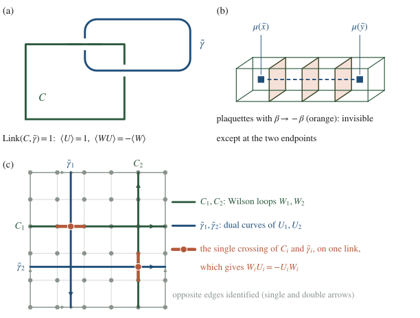
Figure 1. The translation exercise in pictures. (a) A closed dual loop γ̃ linking a Wilson loop (γ̃ passes under C at the upper crossing and over it at the right one): U(γ̃) generates the electric ℤ₂⁽¹⁾ and detects W(C) by linking, (3.1). (b) An open sheet: only its endpoints, the visons, are physical. (c) The spatial torus: γ̃ᵢ crosses Cᵢ once, which gives the algebra (3.2) and the four ground states (3.3).

3.6 What is exact, what is emergent, and where Semester II attaches [Stated — forward references.]

The electric ${\mathbb{Z}}_2^{(1)}$ of (3.1) is exact at every β. In the deconfined phase the visons are gapped, so large vison worldlines are rare and the Wilson loops become topological at long distances: they generate an emergent magnetic ${\mathbb{Z}}_2^{(1)}$ acting on vison worldlines, the magnetic entry of the ${\mathbb{Z}}_N$ BF row of conventions §6 with $d-p-1=1$. At $\Gamma =0$ it is exact on the ground space, where (3.2) says that the generators of each symmetry are charged under the other. Semester II reads this in three ways. (i) Anomaly: the algebra (3.2) is the finite-volume face of the mixed ‘t Hooft anomaly of the electric and magnetic 1-form symmetries, which forces the degeneracy (3.3) wherever both are present (Block 1, Week 2, and Block 2). (ii) Defects: the open sheet of §3.5 is a symmetry defect with a boundary, and the vison is a non-genuine local operator at its end; the sector sum of Week 5 F6 is the gauging of the Ising ${\mathbb{Z}}_2^{(0)}$ (Semester II Week 4). (iii) Condensation: summing the operators $U$ over the 1-cycles of a surface in the deconfined phase condenses visons on that surface, which Semester II Week 13 calls the higher gauging of ${\mathbb{Z}}_2^{(1)}$ and a condensation defect (condensation-defects), and which the group’s research line reads as a Julia–Toulouse condensation restricted to a submanifold. The deconfined phase itself is the ${\mathbb{Z}}_2$ topological-order of the toric-code, whose soluble point is the $\Gamma =0$ Hamiltonian with Gauss’s law imposed energetically (Week 7 §8). These six answers are the template: a translation (Problems 1, 2 and 4⋆ of §13) is complete when it answers (i)–(vi) with a derivation or a precise citation for each.

4. Duality is Poisson resummation

Every duality of the semester was the recipe of Week 2 §7.2: write the compact theory with an explicit integer (or ${\mathbb{Z}}_2$) cochain, resum it with the identities of conventions §3, integrate the original field to obtain a conservation constraint, and solve the constraint on the dual lattice by a dual potential plus winding sectors; the defects reappear only at a second resummation. Table 1 lists every instance. The column of exchanged symmetries is the new content: in each $U(1)$ row the duality exchanges the symmetry whose charged objects are the original excitations with the one whose charged objects are the defects, and the defects, being dynamical, break the second one explicitly.

Duality	Resummed variable; constraint	Dual variables	Defect at the second step	Coupling map	Symmetries exchanged	Derived in
rotor on a ring	winding on the time circle	momentum	—	$\mathcal{T}/2\beta \leftrightarrow 2{\pi }^2\beta /\mathcal{T}$	momentum ↔ winding	Wk 1 §6.1
2d Villain XY	$n\in C^1$; $\delta m=0$	heights, 2 tilts; χ	vortices $v=dn$, points	$\beta \to 1/4{\pi }^2\beta$	shift $U(1{)}^{(0)}$ ↔ winding $U(1{)}^{(0)}$	Wk 3 §§2–6
2d Ising (KW)	${\mathbb{Z}}_2$ loops ↔ walls	dual spins	disorder μ	$\sinh 2K\sinh 2K^{\ast }=1$	${\mathbb{Z}}_2^{(0)}$ ↔ dual ${\mathbb{Z}}_2^{(0)}$	Wk 4 §§3–4
3d ${\mathbb{Z}}_2$ gauge ↔ 3d Ising	closed surfaces ↔ walls	spins on cubes	vison	$\tanh \beta =e^{-2K^{\ast }}$	${\mathbb{Z}}_2^{(1)}$ ↔ Ising ${\mathbb{Z}}_2^{(0)}$	Wk 5 §7
4d ${\mathbb{Z}}_2$ gauge, self-dual	closed surfaces ↔ frustrated dual surfaces	${\mathbb{Z}}_2$ field on ${\Lambda }^{\ast }$	‘t Hooft loop ↔ $W$	$\sinh 2\beta \sinh 2{\beta }^{\ast }=1$	electric ↔ dual electric	Wk 5 §8.3
3d Villain $U(1)$	$n\in C^2$; $\delta b=0$	heights, 3 windings; σ	monopoles $m=dn$, points	$\beta \to 1/4{\pi }^2\beta$; $\frac{e^2}{8{\pi }^2}(\partial \sigma {)}^2$	electric $U(1{)}^{(1)}$ ↔ magnetic $U(1{)}^{(0)}$	Wk 8 §4; Wk 9 §§2–3
4d Villain $U(1)$ (BMK)	$n\in C^2$; $\delta b=0$	$\mathbb{Z}$ gauge field, windings; $\tilde{a}$	monopole loops $j=\star dn$	$\beta \to 1/4{\pi }^2\beta$, $\tilde{e}=2\pi /e$	electric $U(1{)}^{(1)}$ ↔ magnetic $U(1{)}^{(1)}$	Wk 8 §§5–6
3d ${\mathbb{Z}}_2$ gauge–Higgs	surfaces with matter boundaries	the same model	—	$(\beta ,\kappa )\to ({\kappa }^{\ast },{\beta }^{\ast })$	none exact: matter breaks ${\mathbb{Z}}_2^{(1)}$	Wk 13 §4.2
$2+1$ Hamiltonians	bond-algebra maps	TFIM; toric code in fields	—	$\Gamma \leftrightarrow K$; $(h,K,\Gamma ,J)\to (K,h,J,\Gamma )$	as in the Euclidean rows	Wk 5 §7.4; Wk 7 §7.3; Wk 13 §9

Table 1. Every duality of Semester I as one move. The ${\mathbb{Z}}_2$ rows use the ${\mathbb{Z}}_2$ Fourier transform, identity (2.2) of Week 5, in place of Poisson resummation.

Three remarks follow from the table. In every $U(1)$ row the coupling map is $\beta \to 1/4{\pi }^2\beta$, with the $4{\pi }^2$ of Dirac quantization (Week 8 F3). The torus sectors of the second column (tilts, windings, flux sectors) are the part of every duality that bulk formulas elide, and Problem 1 of the take-home final (generalized-symmetries/assessments/final.md; §14) shows that symmetry operators on noncontractible cycles weight them. And the defects of the fourth column are what the modified Villain construction of Semester II Week 12 removes, which makes the second symmetry of each $U(1)$ row exact (conventions §4).

5. Criteria and their failures

The Landau paradigm failed at the places listed in §1, and at each a criterion built on an extended operator took its place. Table 2 lists the criteria, what each measures in the language of §2, and where each fails. The failures carry as much information as the successes: most happen where the symmetry that the criterion measures is explicitly broken or absent, and the others where an exact continuous symmetry cannot break at all, as in the two-dimensional XY model (Mermin–Wagner) and in three-dimensional Maxwell theory (its higher-form version).

Criterion	What it measures	Works for	Fails when, and why	Derived in
local order parameter	breaking of a 0-form symmetry	2d Ising below $T_c$	continuous symmetry in $d=2$ (Mermin–Wagner); every gauge theory (Elitzur); a gauge-fixed $⟨{\sigma }_{\ell }⟩$ is a Wilson line in disguise; the unitary-gauge “Higgs condensate” is at least $\tanh \kappa$ in every phase	Wk 1 §3.5; Wk 4 §3; Wk 5 §3, F2; Wk 13 §2.4
stiffness jump ${\rho }_s/T=2/\pi$	the winding symmetry becoming emergent as vortices bind	2d XY	universal only for the renormalized stiffness; bare couplings are model-dependent	Wk 4 §2; Wk 3 F2
Wilson loop, area or perimeter	electric 1-form symmetry unbroken or broken	pure ${\mathbb{Z}}_2$; compact QED₃ and QED₄; $W_e$ with $e\notin H$	charged matter: perimeter law in every phase, by string breaking; perimeter coefficient non-universal (F2); 3d Maxwell without monopoles: logarithmic potential, the marginal case	Wk 5 §§4–5, 8.1; Wk 10 §5; Wk 11 §5.4; Wk 13 §§2.4, 5; Wk 14 §3.5
’t Hooft loop	the magnetic $U(1{)}^{(1)}$ of 4d compact QED; in 4d ${\mathbb{Z}}_2$, the dual electric ${\mathbb{Z}}_2^{(1)}$ via self-duality	static monopole in the Coulomb phase; 4d ${\mathbb{Z}}_2$, where it is the dual model’s Wilson loop	Villain compact QED with dynamical monopoles: equals 1 identically (F3)	Wk 5 §§8.2–8.3; Wk 11 §5.2
Polyakov loop $⟨L_e⟩$	the center part of ${\mathbb{Z}}_N^{(1)}$ at finite $T$	center-neutral matter; with charge $q$, $L_e$ for $e\notin H$, which vanishes in finite volume and is nonzero in infinite volume only if the residual ${\mathbb{Z}}_r$ breaks	fundamental matter: $⟨L⟩=h_1^{N_{\tau }}\ne 0$ at every coupling	Wk 14 §§4.1–4.3
disorder correlator $⟨\mu \mu ⟩$	the dual ${\mathbb{Z}}_2^{(0)}$	Ising disordered phase; 3d ${\mathbb{Z}}_2$ confined phase	μ is non-genuine: defined with its string, and only in pairs on a torus	Wk 4 §4.2; Wk 5 §7.3, F7
ground-state degeneracy on $T^2$	a broken 1-form symmetry with its clock–shift algebra; topological order	${\mathbb{Z}}_2$: 4; ${\mathbb{Z}}_N$ with charge $q$: $r^2$ in the ${\mathbb{Z}}_r$ Higgs corner, about $N^2$ states in $r^2$ exact sectors in the ${\mathbb{Z}}_N$-deconfined region	exact only at soluble points; elsewhere split at order $L$ for pure ${\mathbb{Z}}_2$ and $N^{\prime }L$ for the $r^2$ sectors (F1)	§3.4; Wk 14 §7
free-energy singularity	any transition	Wegner’s model; the gauge–Higgs lines	Fradkin–Shenker: an analytic path joins Higgs and confinement	Wk 5 §7.1; Wk 13 §§6–7
Fredenhagen–Marcu ratio	screening of charged states, no symmetry	the free-charge phase against the rest	stated with its reference; it is tied to no symmetry	Wk 13 F5

Table 2. The criteria of Semester I and where each fails.

6. The realization of every Semester I symmetry

Table 3 answers question (iii) of §3 for every symmetry of the semester, with the status that question (vi) asks for. Every degree was checked against the master table of conventions §6, and the entries for four-dimensional compact QED follow Table 1 of Week 11.

Theory; symmetry (degree)	Status	First phase	Second phase	Derived in
2d XY; shift $U(1{)}^{(0)}$	exact	low $T$: unbroken, power laws with $\eta =1/2\pi {\beta }_R$ ($1/2\pi \beta$ at the Gaussian level)	high $T$: unbroken, exponential decay	Wk 1 §§3.4–3.5; Wk 4 §2
2d XY; winding $U(1{)}^{(0)}$, $d-2=0$	explicitly broken by vortices	low $T$, $\pi {\beta }_R>2$: breaking irrelevant, emergent	high $T$: relevant, vortex plasma	Wk 3 §6.1; Wk 4 §2
2d Ising; ${\mathbb{Z}}_2^{(0)}$	exact	$K>K_c$: broken	$K<K_c$: unbroken	Wk 4 §3
3d ${\mathbb{Z}}_2$ gauge; electric ${\mathbb{Z}}_2^{(1)}$	exact	$\beta >{\beta }_c$: broken, perimeter law, GSD 4 on $T^2$	$\beta <{\beta }_c$: unbroken, area law	§3; Wk 5 §§4–8
3d ${\mathbb{Z}}_2$ gauge; magnetic ${\mathbb{Z}}_2^{(1)}$	emergent only	deconfined: emergent, visons gapped	confined: visons condensed	§3.6; Wk 5 §7.3
4d ${\mathbb{Z}}_2$ gauge; electric ${\mathbb{Z}}_2^{(1)}$	exact	$\beta >{\beta }_{\mathrm{sd}}$: broken; ‘t Hooft loop area law	$\beta <{\beta }_{\mathrm{sd}}$: unbroken; ‘t Hooft loop perimeter law	Wk 5 §§8.2–8.3
compact QED₃; electric $U(1{)}^{(1)}$	exact	every β: unbroken, area law; no transition	—	Wk 10 §5; Wk 9 §6.2
compact QED₃; magnetic $U(1{)}^{(0)}$	explicitly broken by monopoles	every β: photon gapped (Göpfert–Mack); $m_{\gamma }^2=8{\pi }^2\zeta /e^2$ at weak coupling	— (the monopole-free theory, a different theory, breaks it spontaneously, with the photon as Goldstone boson)	Wk 9 §§5–6; Wk 10 §§3, 7
compact QED₄; electric $U(1{)}^{(1)}$	exact	Coulomb, large β: broken	confining, small β: unbroken	Wk 11 §§4, 5.4
compact QED₄; magnetic $U(1{)}^{(1)}$	explicitly broken; lattice ${\tilde{W}}_m=1$	Coulomb: emergent and broken	confining: explicitly broken	Wk 11 §§5.2, 5.4
compact QED₄ at θ	as above; monopoles carry charge $\theta n_m/2\pi$	condensed dyon $w$: probes with $⟨v,w⟩\ne 0$ confined	probes with $⟨v,w⟩=0$ screened	Wk 12 §§4, 7.2–7.4 (Heuristic; dyons of every label dynamical, as in Cardy–Rabinovici)
${\mathbb{Z}}_2$ gauge–Higgs; electric ${\mathbb{Z}}_2^{(1)}$	explicitly broken by charge-1 matter	Higgs and confined: one phase, no exact symmetry	free-charge region: emergent, topological order	Wk 13 §§2.4, 6; Wk 14 §3.5
${\mathbb{Z}}_N$ with charge $q$; residual ${\mathbb{Z}}_r^{(1)}$, $r=\gcd (N,q)$	exact	confined: unbroken, $W_e$ area law for $e\notin H$	${\mathbb{Z}}_r$ Higgs: broken, GSD $r^2$; ${\mathbb{Z}}_N$-deconfined: broken, ${\mathbb{Z}}_N^{(1)}$ emergent, about $N^2$ states in $r^2$ exact sectors	Wk 14 §§3, 7, Fig. 2(b), F5
thermal lattice; center, the part of ${\mathbb{Z}}_N^{(1)}$ in a time slice	exact for center-neutral matter; $\mathrm{Ann}(H)$ with charge $q$	low $T$: unbroken, $⟨L⟩=0$	high $T$: broken, $⟨L⟩\ne 0$	Wk 14 §§4–5
$U(1)$ with charge-2 matter; residual ${\mathbb{Z}}_2^{(1)}$	exact	superconducting: broken, GSD 4 on $T^2$	—	Wk 14 §8

Table 3. The realization of every symmetry of Semester I. “Broken” means spontaneously broken; “explicitly broken” means that no topological operator exists.

Table 4 relists the extended operators of the semester by their role, which is the dictionary of Gaiotto, Kapustin, Seiberg and Willett in the form Semester II opens with.

Operator	First derived	Role in Semester II language
Ising seam on a closed dual curve	Wk 4 §4.1	generator of ${\mathbb{Z}}_2^{(0)}$ in $d=2$
Kadanoff–Ceva μ	Wk 4 §4.1	endpoint of an open seam; a non-genuine local operator
Kramers–Wannier operator $D$	Wk 4 §4.4	non-invertible topological line at $K_c$ (Semester II Week 13)
vortex operator $e^{i\chi }$, $d=2$	Wk 3 §6.1	charged local operator of the winding $U(1{)}^{(0)}$
Wilson loop $W(C)$	Wk 5 §2.2; Wk 6 §1.2	charged line of the electric 1-form symmetry
closed flipped or twisted sheet $U(\tilde{\Sigma })$	Wk 5 §8.1; Wk 11 §5.1; Wk 14 §3.1	generator of the electric 1-form symmetry
vison μ, $d=3$	Wk 5 §7.3	endpoint of an open sheet; the dual Ising spin
monopole operator $e^{iq\sigma }$, $d=3$	Wk 8 §4.5; Wk 9 §5.1	charged local operator of the magnetic $U(1{)}^{(0)}$
magnetic flux $\exp (i\alpha {\oint }_{\Sigma }F/2\pi )$ on a closed surface	Wk 9 §5.1; Wk 11 §5.2	generator of the magnetic $(d-3)$-form symmetry, explicitly broken by monopoles
’t Hooft loop $\tilde{W}(\tilde{C})$, $d=4$	Wk 5 §8.2 for ${\mathbb{Z}}_2$; Wk 11 §5 for $U(1)$	for $U(1)$, charged line of the magnetic $U(1{)}^{(1)}$, screened in Villain compact QED; for ${\mathbb{Z}}_2$, boundary of an open electric sheet, charged under the dual electric ${\mathbb{Z}}_2^{(1)}$ of the self-dual description, which has no generator in the original variables
Polyakov loop $L_e$	Wk 14 §4.1	charged under the center part of ${\mathbb{Z}}_N^{(1)}$; an order parameter only where that part is exact
twists and flux sectors	Wk 3 F3; Wk 8 F4; Wk 14 §6	temporal twists: symmetry operators on noncontractible cycles; spatial twists: flux sectors that no operator creates

Table 4. The extended operators of Semester I, reorganized. Each is a symmetry operator, a charged object, or the boundary of an open symmetry operator.

7. The course map

Figure 2 places the four recurring threads of the syllabus (its §8) and the question of Semester I against the weeks. Read by rows, it shows that each thread was built before it was used: Poisson resummation is derived in Weeks 1–2 and fired in Weeks 3–8; the symmetry operators of Weeks 4–5 return in Weeks 9–11 and 14; and the condensation thread runs without interruption from Week 9 to Week 13. Read by columns, it tells a student where to look when a problem names a week; for the take-home final, the diagnostic map in its package (§14) does the same problem by problem.

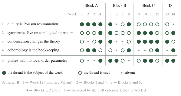
Figure 2. The course map: the four threads of the syllabus and the question of Semester I (row 5) against the fourteen weeks, with the Semester II blocks in which each continues.

8. Subtleties and fine print

F1 — Finite versus infinite volume. In finite volume no symmetry of any degree is spontaneously broken. On the $L\times L$ torus the ground states of §3.4 are exact eigenstates of $U_1$ and $U_2$, and the four sectors are split at order $(\Gamma /K{)}^L$; broken symmetry is the statement that the splitting vanishes as $L\to \infty$ and that the states of definite holonomy, in which $⟨W_i⟩\ne 0$, are the ones that cluster. The limits are taken in the order of Week 5 F1, the volume first and the loops afterwards. For a 0-form symmetry the splitting of the ordered doublet requires an operator on all of space, $L^D$ sites, and for a 1-form symmetry an operator on a closed curve, $L^{D-1}$ links (Week 14 §7.2); in both cases it is exponentially small in a power of $L$, and for the 1-form symmetry the number of sectors depends on the topology of space, $r^{b_1}$ (Week 14 §7.1). In the Euclidean path integral on a torus, (3.1) holds for sheets that bound. On a noncontractible cycle $⟨U⟩$ differs from 1, since the operator is then a twisted boundary condition that weights the flux sectors (Week 3 F3; Problem 1(d) of the take-home final in generalized-symmetries/assessments/final.md), as the reversed seam of the Ising model gives $⟨\eta ⟩=Z_{\mathrm{AP}}/Z_{\mathrm{P}}$ (Problem 1); Problem 5⋆ computes it for Wegner’s model.

F2 — The perimeter-law normalization. The coefficient μ of a perimeter law is a self-energy of the probe: it depends on the lattice action and on the corners of $C$, nothing universal attaches to its value (Week 5 F3), and in the continuum it diverges as $|C|/a_{\mathrm{lat}}$. The SSB criterion therefore refers to $⟨W(C)⟩e^{\mu |C|}$ with a counterterm local on $C$, which removes perimeter and corner terms and can never remove an area term, since a counterterm local on $C$ grows at most like $|C|$. The invariant tools are the Creutz ratio, which cancels perimeter, corner and constant terms exactly (Week 5 F3; Week 6 §6), and, with matter, the Fredenhagen–Marcu ratio, whose square root cancels the self-energy of an open line (Week 13 F5). “Perimeter law” in Tables 2 and 3 means “no area term”.

F3 — The Villain ‘t Hooft loop. In the Villain theory with dynamical monopoles the integer twisted sheet bounded by $\tilde{C}$ is a relabeling of the summed integers, so the integer ‘t Hooft loop equals 1 identically and the magnetic symmetry is explicitly broken in every phase (Week 11 §5.2). The entries of Tables 2–4 that give ‘t Hooft loops of $U(1)$ theories a perimeter or an area law refer to a static monopole probe with its Coulomb field, to the emergent magnetic symmetry of the Coulomb phase, or to the monopole-free theory, in which $dn=0$ is imposed and the loop becomes the Wilson loop of the dual photon (Semester II Week 12). In ${\mathbb{Z}}_2$ gauge theory the Bianchi identity holds identically, and the ‘t Hooft loop of Week 5 §8.2 is a well-defined line operator in $d=4$, mutually non-local with the Wilson loop (Week 5 §8.3). It is charged under the electric ${\mathbb{Z}}_2^{(1)}$ of the self-dual description, which has no generator in the original variables, since the product of ${\sigma }_P$ over a closed surface is identically 1 (Week 5 F6); the magnetic symmetry of the ${\mathbb{Z}}_2$ BF row is a 2-form symmetry with surface charged objects (Problem 3).

F4 — Explicit versus spontaneous breaking. The SSB criterion presupposes an exact symmetry. With charged dynamical matter the would-be symmetry operator acquires local factors on the region it bounds and a perimeter law in its own size (Week 14 §3.1; Week 13 Problem 4⋆), Wilson loops obey a perimeter law in every phase (Week 13 §2.4), and nothing follows about the realization of any symmetry. With charge-$q$ matter in ${\mathbb{Z}}_N$ the exact part is $\mathrm{Ann}(⟨q⟩)\cong {\mathbb{Z}}_{\gcd (N,q)}^{(1)}$ (Week 14 §3), and the criterion applies to it alone. The Polyakov loop is likewise an order parameter only for the part of the center that the matter leaves exact: all of ${\mathbb{Z}}_N$ for center-neutral matter, nothing for fundamental matter, where $⟨L⟩\ne 0$ at every coupling (Week 14 §4.3). Emergent symmetries (the magnetic ones of the Coulomb and deconfined phases, the winding symmetry of the BKT phase) organize long-distance physics and carry no exact theorem.

F5 — Local observables still see the transitions. A phase transition without a local order parameter is still visible to local observables: the plaquette energy of Wegner’s model is singular at ${\beta }_c$, with the specific-heat singularity of the 3d Ising model (Week 5 §11), and every transition of Tables 2 and 3 is a free-energy singularity. What is absent is a local operator that vanishes by symmetry in one phase and not in the other.

F6 — Which dimension. Every degree in this note uses $d$ for the spacetime dimension. A $p$-form symmetry has operators of dimension $d-p-1$ in spacetime and $D-p$ in a spatial slice, and charged objects of dimension $p$. The magnetic symmetry of a $U(1)$ gauge field is $(d-3)$-form, a 0-form symmetry with local monopole operators in $d=3$ and a 1-form symmetry with ‘t Hooft lines in $d=4$. Evaluating a rule written for the spatial dimension at the spacetime dimension is the origin of erratum E1 (conventions, course-local override), and every symmetry statement of the final is checked against the master table.

9. Common misconceptions

• “Generalized symmetry is a reformulation with no new content.” It is tempting because every result of Semester I was derived without the language, and the tables of this week relabel those results. The language has consequences that no single calculation of the semester stated. The degeneracy (3.3) follows from the algebra (3.2) of symmetry operators and charged lines alone, so it holds wherever that algebra holds on the ground space, including points with no soluble limit. Two phases in which an exact symmetry is realized differently must be separated by a transition, which is why the $N=6$, $q=4$ diagram of Week 14 (its Figure 2) needs a transition line while the charge-1 diagram does not (Week 14 §3.5). The higher-form Coleman–Mermin–Wagner theorem constrains every three-dimensional model at once: no continuous 1-form symmetry breaks there (conventions §6). And with fundamental matter the absence of any exact symmetry is the invariant content of Fradkin–Shenker complementarity. Semester II adds ‘t Hooft anomalies, which constrain phases through the algebra of the operators without any dynamical calculation.
• “The ‘t Hooft loop generates the magnetic 1-form symmetry.” It is tempting because both carry the adjective magnetic and the ‘t Hooft loop is built from a twisted sheet. The generator of the magnetic $U(1{)}^{(1)}$ of four-dimensional Maxwell theory is the surface operator $\exp (i\alpha {\oint }_{\Sigma }F/2\pi )$ on a closed 2-surface, and the ‘t Hooft line is its charged object, detected by linking. The twisted sheet on a closed surface generates the electric symmetry, and the ‘t Hooft loop is the boundary of an open one (Week 11 §§5.1–5.2; §3.5 for ${\mathbb{Z}}_2$). Its first appearances are Week 5 §8.2 for ${\mathbb{Z}}_2$ and Week 11 §5 for $U(1)$.
• “The Polyakov loop is the order parameter of confinement whatever the matter.” It is tempting because in pure gauge theory the center symmetry forces $⟨L⟩=0$ in the confined phase exactly. With fundamental matter the center symmetry is explicitly broken and $⟨L⟩=h_1^{N_{\tau }}\ne 0$ at every coupling, so the Polyakov loop separates nothing; it is an order parameter for center-neutral matter, and with charge-$q$ matter only the loops $L_e$ with $e\notin H$ remain order parameters: $⟨L_e⟩$ vanishes identically in finite spatial volume and is nonzero in infinite volume only if the residual ${\mathbb{Z}}_r$ breaks spontaneously, which it can at high temperature (Week 14 §§4.1, 4.3).

10. Historical note

Gaiotto, Kapustin, Seiberg and Willett (2014) wrote in continuum language, with differential forms and background gauge fields. They defined a $q$-form symmetry by topological operators of codimension $q+1$, showed that the group is abelian for $q\ge 1$, coupled the symmetries to $(q+1)$-form backgrounds, and discussed gauging, ‘t Hooft anomalies and spontaneous breaking, including the higher-form Coleman–Mermin–Wagner theorem; their examples include Maxwell theory and ${\mathbb{Z}}_N$ gauge theory, the continuum versions of our Weeks 5, 8–11 and 14. The ingredients were older, and Semester I read them in their original form: Wegner’s loop correlations and duality (1971), Wilson’s area-law criterion (1974), Polyakov’s monopole plasma (1975–77), the duality of Banks, Myerson and Kogut (1977), and ‘t Hooft’s classification of phases by electric and magnetic flux (1978), whose temporal twists are symmetry operators of the center 1-form symmetry. What the 2014 paper supplied was one definition that covers all of them and puts the loop criteria on the footing of Landau’s.

11. What to take away

1. A $p$-form symmetry is a family of topological operators on closed $(d-p-1)$-dimensional submanifolds that act by linking on $p$-dimensional charged objects [Stated; model case Proved]. On the lattice topological invariance is always a change of variables; physically, a symmetry operator can be moved without being noticed, except by what it links.
2. Wegner’s theory, translated: an exact electric ${\mathbb{Z}}_2^{(1)}$ with Wilson lines as charged objects, spontaneously broken in the deconfined phase with four ground states on $T^2$ forced by the clock–shift algebra (3.2), unbroken in the confined phase; the vison is the endpoint of an open symmetry operator [Proved and Computed].
3. Every duality of the semester is Poisson (or ${\mathbb{Z}}_2$ Fourier) resummation followed by a constraint solved on the dual lattice, with $\beta \to 1/4{\pi }^2\beta$ in each $U(1)$ row. It exchanges a symmetry with a dual one whose charged objects are the defects, which break it explicitly.
4. Each criterion measures the realization of one symmetry. It fails where that symmetry is explicitly broken (Wilson and Polyakov loops with fundamental matter, ‘t Hooft loops with dynamical monopoles, local order parameters in gauge theories) and where a continuous symmetry cannot break at all (the two-dimensional XY model, three-dimensional Maxwell theory).
5. Semester I’s phases are classified by Table 3. Where no exact symmetry survives, as with fundamental matter, no symmetry distinction between phases exists, and the deconfined phases are told apart by topological order, whose Semester I fingerprint is the degeneracy on the torus.

12. Looking ahead: Semester II

Semester II opens (Block 1) with the definitions of §2: Week 1 defines symmetries as topological operators, Week 2 builds ${\mathbb{Z}}_N$ gauge theory as BF theory and constructs the operators whose algebra (3.2) we used, Week 3 makes the SSB criterion precise, and Week 4 defines gauging, which turns the forward references of §§2 and 3.6 into theorems. Block 2 treats ‘t Hooft anomalies, including the mixed anomaly at θ = π that grows out of Week 12; Block 3 solves the toric code, the deconfined phase of §3; Block 4 makes the dualities of Table 1 exact with the modified Villain construction (Week 12) and turns the Kramers–Wannier operator of Week 4 §4.4 into a non-invertible defect (Week 13). Block 5 returns to the residual symmetry of Week 14 through higher-gauging walls, the setting of the group’s manuscript in preparation, and the master-project.

13. Problem set

Problems 1–3 are the classroom core and are solvable from this note and the weeks it cites; Problems 4⋆ and 5⋆ are self-study consolidation, each with a hint; Problem 6⋆⋆ is a research extension that states what is known, what is explored, its sources and what counts as completion. No problem shares a part with the take-home final of §14; the parts of the final that may cite this note, checkpoints included, are listed in the rules of its paper.

Core problems (everyone).

1. Translate the two-dimensional Ising model. (Extends §3 to $p=0$.) For $Z={\sum }_s\exp \left(K{\sum }_{⟨xy⟩}{s}_x{s}_y\right)$ on the square lattice: (a) let $\eta (\tilde{\gamma })$ reverse $K$ on the bonds crossed by a closed dual curve $\tilde{\gamma }$ that encloses the set of sites $R$, and show that $⟨\eta (\tilde{\gamma })⟩=1$ and $⟨\eta (\tilde{\gamma })s_x{s}_y⟩=(-1{)}^{[x\in R]+[y\in R]}⟨s_x{s}_y⟩$; check the degree against §2. (b) Give the realization in the two phases, and the ground states of the transverse-field chain $H(g)$ of Week 4 §4.4 on a ring of $N$ sites at $g\ll 1$ and $g\gg 1$, with the order in $g$ at which the two ordered states split. (c) Identify the open seam and its endpoints, and say which operator condenses in each phase. (d) Answer question (vi) of §3 for this model.

2. Translate compact QED₄ at θ ≠ 0. (Extends §3 to a θ-term; Weeks 11–12.) In the Hamiltonian slice of four-dimensional compact QED with a θ-term: (a) show that $\exp (i\alpha \hat{N}(\Sigma ))$, with $\hat{N}(\Sigma )={\oint }_{\Sigma }(E/e^2-\theta B/4{\pi }^2)\cdot dS$ on a closed spatial surface Σ, is the electric symmetry operator: it measures the integer $n_e$ of the lines that Σ encloses, is unchanged when a dynamical monopole crosses Σ, and is $2\pi$-periodic in α, while the flux of $E/e^2$ alone measures $q_e=n_e+\theta n_m/2\pi$ (Week 12 §§4.1–4.2); give the magnetic symmetry operator and its status from Table 3. (b) List the charged lines, Wilson lines $(n_e,0)$, ‘t Hooft probes $(0,n_m)$ and dyonic lines $(n_e,n_m)$, with their charges under both symmetries, and show how the labels move under $\theta \to \theta +2\pi$ (Week 12 §5). (c) At strong coupling Week 12 §7.3 lets the magnetic dyon $(0,1)$ condense for $-\pi <\theta <\pi$ and $(-1,1)$ for $\pi <\theta <3\pi$, in the setting of Cardy and Rabinovici where dyons of every label are dynamical (in pure compact QED₄ the only dynamical magnetic objects are the monopoles $(0,1)$); apply the rule of Week 12 §7.2 to the probes $(1,0)$, $(0,1)$ and $(-1,1)$ on each side, and say what changes at θ = π and what does not. (d) Answer question (vi) of §3 for this theory.

3. A form-degree drill. (Extends §2.) For the compact scalar and the $U(1)$ gauge field in $d=3$ and $d=4$, and for ${\mathbb{Z}}_2$ BF theory with a 1-form gauge field in $d=3$ and $d=4$, list each symmetry with its degree, the dimension of its charged objects, the dimension of its operators in spacetime and in a spatial slice, and, for the continuous ones, whether the higher-form Coleman–Mermin–Wagner theorem allows spontaneous breaking. Mark the entries that Semester I realized and give the week.

Starred problems (Ph.D. expected; ambitious M.Sc. encouraged).

4⋆. Translate the four-dimensional ℤ₂ gauge theory. Carry out the six steps of §3 for Wegner’s model in $d=4$: the ground-state degeneracy on the spatial $T^3$ at both soluble points, with the three clock–shift pairs that force it; the realization of ${\mathbb{Z}}_2^{(1)}$ on either side of ${\beta }_{\mathrm{sd}}$; and the role of the ‘t Hooft loop under the self-duality of Week 5 §8.3. (Hint: (7.1) of Week 14 with $N=2$, $q\equiv 0$ and $b_1(T^3)=3$; in three spatial dimensions the electric symmetry operators live on closed dual surfaces.)

5⋆. The noncontractible symmetry operator as a diagnostic. (Extends §3.4 and F1.) On the $L\times L\times L_{\tau }$ Euclidean torus of the 3d ${\mathbb{Z}}_2$ gauge theory, let $\tilde{\gamma }$ be a dual loop that winds a spatial cycle at fixed Euclidean time. (a) Show that $⟨U(\tilde{\gamma })⟩=\mathrm{Tr}(U{\mathcal{T}}^{L_{\tau }})/\mathrm{Tr}{\mathcal{T}}^{L_{\tau }}$, with $\mathcal{T}$ the transfer matrix of Week 7 and $U$ the operator of §3.1, and use §3.4 to find its limit as $L_{\tau }\to \infty$ in each phase, at fixed $L$ and when $L\to \infty$ first (which sector is lowest at fixed $L$ follows from the sign of the order-$L$ splitting, or from (b)). (b) At weak coupling, show that the reversed plaquettes cannot all be satisfied, that the cheapest configurations carry a frustrated dual loop homologous to $\tilde{\gamma }$, and that a dilute gas of such wrapped vison worldlines gives $⟨U(\tilde{\gamma })⟩\simeq \tanh (L{L}_{\tau }{e}^{-2\beta L})$ at leading order; interpret the two limits of (a). (c) At strong coupling, show that $1-⟨U(\tilde{\gamma })⟩$ is controlled by the smallest closed surfaces that $\tilde{\gamma }$ pierces an odd number of times, and compare the two phases with $⟨\eta ⟩=Z_{\mathrm{AP}}/Z_{\mathrm{P}}$ of Problem 1. (Hint: in the untwisted partition function the wrapped vison loops of this class come in even numbers, in the twisted one in odd numbers.)

⋆⋆ problems (research extension; optional).

6⋆⋆. The toric code in two fields, translated. What is known. The toric code in electric and magnetic fields is the Hamiltonian form of the ${\mathbb{Z}}_2$ gauge–Higgs model (Week 13 §9); its phase diagram, with a deconfined region bounded by two continuous lines that meet at a multicritical point and a first-order segment on the self-dual line, was mapped by Tupitsyn, Kitaev, Prokof’ev and Stamp, Phys. Rev. B 82 (2010) 085114 [arXiv:0804.3175] (Week 13 §7). What is explored. The realization of the exact and emergent symmetries in each region. Sources: Week 13 §§7, 9 and F5; Week 14 Figure 2(a) and F5; the paper of Tupitsyn et al. Completion: a table giving, for each region and each line, the status (exact, explicitly broken, emergent) and the realization of the electric and magnetic ${\mathbb{Z}}_2^{(1)}$, each entry justified by a limit computed in Weeks 5, 13 or 14; the action of the $e$–$m$ duality on the table; and one paragraph, labelled heuristic, on what distinguishes the free-charge phase from the Higgs–confined phase in the absence of any exact symmetry.

Self-study answer checkpoints

These checkpoints cover the core problems; starred and ⋆⋆ problems remain source-led.

1. The Ising translation. The decisive step is the change of variables $s_x\to -s_x$ for $x\in R$, which restores every reversed bond, since exactly the bonds crossed by $\tilde{\gamma }$ have one end in $R$; it leaves the measure invariant and multiplies $s_x{s}_y$ by $(-1{)}^{[x\in R]+[y\in R]}$. The operator is topological, with group ${\mathbb{Z}}_2$, on a closed support of dimension $d-p-1=1$: a 0-form symmetry with the local charged operator $s_x$. It is broken for $K>K_c=0.440687$ and unbroken below; on the ring the states $|\Uparrow ⟩\pm |\Downarrow ⟩$ at $g\ll 1$ split at order $g^N$, since all $N$ spins must flip, and the ground state at $g\gg 1$ is unique. The open seam has the disorder operators μ at its ends, with $⟨\mu \mu {⟩}_K=⟨ss{⟩}_{K^{\ast }}$, so μ condenses in the disordered phase (Week 4 §§4.1–4.2). For (vi): the symmetry is exact, and the Kramers–Wannier map exchanges its broken and unbroken phases, which is the gauging of ${\mathbb{Z}}_2^{(0)}$ with the dual ${\mathbb{Z}}_2^{(d-0-2)}={\mathbb{Z}}_2^{(0)}$ (forward reference); at $K_c$ it becomes the non-invertible line $D$ of Week 4 §4.4. Common failure mode: calling μ the symmetry operator, or expecting $⟨\eta ⟩$ to vanish in the broken phase. For bounding $\tilde{\gamma }$, $⟨\eta ⟩=1$ in every phase; on a torus a noncontractible $\tilde{\gamma }$ is the antiperiodic boundary condition of Week 4 §3.4, and $⟨\eta ⟩=Z_{\mathrm{AP}}/Z_{\mathrm{P}}$ tends to 0 in the ordered phase, where a domain wall of length $L$ is forced, and to 1 in the disordered one.
2. Compact QED₄ at θ. (a) The θ-modified Gauss law of Week 12 §4.1 makes $\nabla \cdot (E/e^2-\theta B/4{\pi }^2)$ the density of the integers $n_e$, so $\hat{N}(\partial V)$ is the total $n_e$ inside $V$, an integer by compactness (Week 12 §4.2), and $\exp (i\alpha \hat{N})$ multiplies $W_q$ by $e^{iq\alpha \mathrm{Link}}$: an electric $U(1{)}^{(1)}$ with α defined mod $2\pi$. A dynamical monopole crossing Σ changes $\oint E/e^2$ by $\theta /2\pi$ and $\oint \theta B/4{\pi }^2$ by the same amount, so $\hat{N}$ is unchanged, while the flux of $E/e^2$ alone is not topological. The magnetic operator $\exp (i\alpha {\oint }_{\Sigma }F/2\pi )$ counts $n_m$ and is explicitly broken by the dynamical monopoles (Table 3; F3). (b) The line $(n_e,n_m)$ has charge $n_e$ under the electric symmetry, magnetic charge $n_m$ and physical charge $q_e=n_e+\theta n_m/2\pi$; at $\theta +2\pi$ the line labelled $(n_e,n_m)$ carries the charges of $(n_e+n_m,n_m)$ at θ, so the set of line labels returns, shifted (conventions §10); the dynamical spectrum returns only if dyons of every label are dynamical, and with monopoles alone the lattice θ-term is not $2\pi$-periodic. (c) With $w=(0,1)$ the pairing is $⟨v,w⟩=n_e$, which confines $(1,0)$ and $(-1,1)$ and screens $(0,1)$; with $w=(-1,1)$ it is $n_e+n_m$, which confines $(1,0)$ and $(0,1)$ and screens $(-1,1)$ (Week 12 §7.3). The Wilson probe is confined on both sides; what changes at θ = π is which line with $n_m\ne 0$ is screened, and at θ = π the two condensates tie and are exchanged by ${\mathrm{CP}}_{\theta =\pi }:(n_e,n_m)\to (-n_e-n_m,n_m)$ [Heuristic]. (d) In the pure theory the dynamical objects are monopoles with $n_e=0$, so the electric symmetry of (a) is exact at every θ and the magnetic one is explicitly broken; the oblique phases of Week 12 §7 belong to models with dynamical dyons of every $n_e$ (Week 12 §7.4 and its references), in which the electric symmetry is explicitly broken too and the phases are told apart by the pattern of (c). Semester II Week 6 reads the tie at θ = π as a mixed ‘t Hooft anomaly involving CP (forward reference; GKKS). Common failure mode: taking the flux of $E/e^2$ as the symmetry charge, which the dynamical monopoles change by θ/2π.
3. The form-degree drill. Compact scalar: shift, 0-form, charged $e^{iq\theta }$, operators of dimension $d-1$ in spacetime and $D$ in space, breaking allowed in $d=3,4$; winding, $(d-2)$-form, charged vortex lines in $d=3$ and vortex sheets in $d=4$, operators $\exp (i\alpha \oint d\theta /2\pi )$ on closed curves in both, breaking forbidden in both ($d-2\ge d-2$). $U(1)$ gauge field: electric 1-form, Wilson lines, operators of dimension $d-2$ (curves in $d=3$, surfaces in $d=4$), breaking forbidden in $d=3$ and allowed in $d=4$; magnetic $(d-3)$-form, local monopole operators and closed-surface operators in $d=3$, ‘t Hooft lines and closed-surface operators in $d=4$, breaking allowed in both. ${\mathbb{Z}}_2$ BF: electric 1-form with Wilson lines and operators of dimension $d-2$; magnetic $(d-2)$-form with charged objects of dimension $d-2$ (vison worldlines in $d=3$, surfaces in $d=4$) and the Wilson lines as operators; the theorem does not apply to discrete groups. Realized in Semester I: the $d=3$ compact scalar as the dual photon of Weeks 8–10, whose shift symmetry is the magnetic $U(1{)}^{(0)}$; the $U(1)$ gauge field in $d=3$ (Weeks 9–10) and $d=4$ (Week 11); and the ${\mathbb{Z}}_2$ rows as the deconfined limit of Wegner’s model in $d=3$ and $d=4$ (Week 5; §3), whose lattice form keeps only the electric symmetry exact. Common failure mode: taking the operator dimension for the degree, or $(d-2)$ for the magnetic degree of a gauge field.

14. The take-home final

The take-home final is handed out at the end of this week and is due fourteen days later; it counts for 20% of the Semester I grade (syllabus §5). It has five problems of 20 points each: Problem 1, one engine, two chains; Problem 2, string breaking in the ℤ₂ gauge–Higgs model; Problem 3, a Polyakov estimate and the energy–entropy balance; Problem 4, the Kramers–Wannier operator on the periodic chain; and Problem 5⋆, the residual 1-form symmetry. The core track attempts Problems 1–4, graded out of 80 points and rescaled to 100; the starred track attempts all five, out of 100. The notes of Weeks 1–15, conventions and the sources they cite are allowed material. This note is among them, and the rules of the paper list the clauses that may cite it and say where small numerical checks are allowed. The final package (the student paper with its rules and citation list, the instructor key with point rubric and common errors, and the diagnostic map back to the notes) is a separate document in generalized-symmetries/assessments/final.md; this note does not contain it.

---

Notes prepared for the generalized-symmetries course, Semester I Block D — the close of Semester I. Rewritten to the note-quality-template standard on 2026-09-29 (first draft 2026-07-01). Last revised 2026-10-04.