Week 6 — Wilson’s Formulation: Compact Groups, Haar Measure, Strong Coupling

Wegner’s ${\mathbb{Z}}_2$ gauge theory of Week 5 already contained the logic of lattice gauge theory: variables on links, an action on plaquettes, no local order parameter, and a Wilson loop whose strong-coupling expansion tiles a surface. This week we replace the sign on each link by an element of a compact Lie group, as Wilson did in 1974 to regulate electrodynamics and Yang–Mills theory. One new tool does all the work. We integrate each link over the group with its invariant (Haar) measure and expand the plaquette weight in characters, exactly as Week 1 expanded the rotor chain in the characters of U(1); the strong-coupling series then becomes a sum over surfaces, and the area law comes out for every compact group, with a coefficient that we compute for U(1), SU(2) and SU(N). Whether this confinement survives at weak coupling depends on the group and on the dimension: compact U(1) confines at every coupling in $d=3$ (Weeks 9–10) and has a Coulomb phase in $d=4$ (Week 11), while for SU(N) in $d=4$ the expectation, supported by Monte Carlo and unproven, is that no transition separates strong from weak coupling. Week 7 turns the same lattice into a Hamiltonian.

How to use this chapter

• In class: derive at the board, in this order, the invariance of the Haar measure and the rules (G0)–(G2) of §2.3 (the Schur argument takes five lines), the SU(2) class measure of §2.2, the coefficient ${\tilde{c}}_{1/2}=I_2(\beta )/I_1(\beta )=\beta /4+O({\beta }^3)$ of §3.3 and the SU(N ≥ 3) coefficient $\beta /2N^2$ of §3.4; then the 2×2 loop link by link (§4.1, Figure 1), the tiling rule (§4.2) and the first correction $\sigma =-\ln {\tilde{c}}_F-2(d-2){\tilde{c}}_F^4$ (§4.3, Figure 2). In the second lecture: the continuum limit with $\beta =2N/g^2$ and $\beta =1/e^2$ (§5), Creutz ratios (§6) and roughening (§7.3). Problems 1–4 are the classroom core.
• For self-study: the Euler-angle chart of §2.2, §3.5, the remaining fine print (§§7.1–7.2 and 7.4–7.7) and §§8–9. The one calculation to do alone is Problem 1, the 1×2 loop by hand, followed by the same computation with one tile reversed, which vanishes for SU(3) and does not vanish for SU(2).
• Instructor checkpoint: the SU(2) coefficient. Since $\mathrm{tr}U=\mathrm{tr}{U}^{†}$ for SU(2), both halves of $\mathrm{Re}\mathrm{tr}U$ feed the spin-½ character and ${\tilde{c}}_{1/2}\simeq \beta /4$; setting $N=2$ in $\beta /2N^2$ gives $\beta /8$, off by a factor 2 (§3.3). The second trap is the counting of powers of N in a tiling: every link integral costs $1/N$ and every site of the surface returns a factor N, and a student who forgets the sites is off by $N^{-V}$, for instance $N^{-9}$ for the 2×2 loop (§4.2). The third is the coupling: $\beta =2N/g^2$ belongs to SU(N), and U(1) has $\beta =1/e^2$ (§5).

0. Reading

Primary: Wilson, Phys. Rev. D 10 (1974) 2445, §III (the lattice formulation, with the gauge field as an angular variable and no gauge fixing) and §IV (the strong-coupling expansion and the area law). Kogut, Rev. Mod. Phys. 55 (1983) 775: §III for the 2×2 SU(2) loop at strong coupling with the two Haar integrals of §2.3 (its Figs. 23–24), §IV.A for character expansions and the “house” correction of the ${\mathbb{Z}}_2$ loop, §§V.B–V.C for the universal $1/R$ term and roughening.

Secondary:

• Kogut, Rev. Mod. Phys. 51 (1979) 659, §V.D (the ${\mathbb{Z}}_2$ loop), §VI.A–B (abelian lattice gauge theory, its strong-coupling area law and phase diagrams) and §VIII.A–B (the SU(2) theory, its classical continuum limit, and whether strong and weak coupling are connected).
• Drouffe & Itzykson, Phys. Rep. 38 (1978) 133, §3.1 (selection rules of the character expansion) and Appendix C (group measures for ${\mathbb{Z}}_n$, U(1), SU(2) and U(n)).
• Creutz, Phys. Rev. D 21 (1980) 2308: the first Monte Carlo study of SU(2), with the ratios of §6.

Optional research reading: Osterwalder & Seiler, Ann. Phys. 110 (1978) 440 (convergence of the strong-coupling expansion and the area law at small β for every compact group); Göpfert & Mack, Commun. Math. Phys. 82 (1982) 545 (3d U(1) with the Villain action confines at every coupling); Guth, Phys. Rev. D 21 (1980) 2291, and Fröhlich & Spencer, Commun. Math. Phys. 83 (1982) 411 (the Coulomb phase of 4d U(1)); Svetitsky & Yaffe, Nucl. Phys. B 210 (1982) 423 (for §7.6).

Proof-status labels as in Week 1. Every sign and normalization comes from conventions §4, and every reference from bibliography-and-paper-map.

1. From ${\mathbb{Z}}_2$ to a compact group

1.1 The question

Static sources in a representation r of the gauge group G, held at distance R for a Euclidean time T, feel a potential $V(R)$ that we read off the Wilson loop, $⟨W_r(C)⟩\sim e^{-V(R)T}$ for the $R\times T$ rectangle C. If V grows linearly, the sources are confined. In Week 5 the group was ${\mathbb{Z}}_2$ and the strong-coupling answer was $⟨W⟩\simeq (\tanh \beta {)}^A$. For a compact Lie group three things change. The sum over the two values of a sign becomes an integral over G, which must respect the group multiplication (the Haar measure, §2). The plaquette weight expands in all irreducible representations of G (the characters, §3). And the rule “a link integrates to zero unless it appears an even number of times” becomes “a link integrates to zero unless the representations it carries contain the singlet”, which forces tiled surfaces (§4). The two groups of physical interest are U(1), the lattice regulator of compact electrodynamics whose monopoles drive Block C, and SU(N), the lattice regulator of Yang–Mills theory (lattice-gauge-theory, confinement).

1.2 Link variables and what is gauge invariant

On each oriented link ${\ell }_{\mu }(x)$ from x to $x+\hat{\mu }$ we place $U_{\mu }(x)\in G$; the reversed link carries $U_{\mu }(x{)}^{-1}=U_{\mu }(x{)}^{†}$. A gauge transformation assigns $g_x\in G$ to every site and acts as

$$U_{\mu }(x)⟶g_x{U}_{\mu }(x)g_{x+\hat{\mu }}^{-1}.$$

The ordered product $U_{\gamma }$ along a path γ transforms as $g_{\mathrm{start}}{U}_{\gamma }{g}_{\mathrm{end}}^{-1}$, so the holonomy of a closed loop C based at x transforms by conjugation, $U_C\to g_x{U}_C{g}_x^{-1}$. It is gauge covariant, and for a non-abelian group its invariant functions are the class functions, spanned by the characters ${\chi }_r(U_C)=\mathrm{tr}{D}^r(U_C)$ of the irreducible representations $D^r$ of dimension $d_r$. The Wilson loop in representation r is

$$W_r(C)=\frac{1}{d_r}{\chi }_r(U_C),$$

normalized to 1 on the trivial configuration. The plaquette holonomy, with the orientation of conventions §1 (bottom, right, top reversed, left reversed), is

$$U_P=U_{\mu }(x)U_{\nu }(x+\hat{\mu })U_{\mu }(x+\hat{\nu }{)}^{†}{U}_{\nu }(x{)}^{†},$$

and the same remarks apply to it: $U_P$ is conjugated at its base corner under a gauge transformation, it is conjugated by a link when the base corner is moved, and it becomes $U_P^{†}$ when the orientation is reversed. Only its class is observable. For U(1), $U_{\mu }(x)=e^{i{a}_{\mu }(x)}$ with $a_{\mu }(x)\in (-\pi ,\pi ]$, the plaquette is $U_P=e^{i(da{)}_P}$ with the coboundary of Week 2, conjugation is trivial and $U_P$ itself is invariant; with $g_x=e^{-i{\lambda }_x}$ the transformation above is $a\to a+d\lambda$ of conventions §4, and the charge-q loop is $W_q(C)=e^{iq{\sum }_{C}a}$ (conventions §6). In the continuum, $U_{\ell }=\mathcal{P}\exp (i{\int }_{\ell }A)$ with $A=A^a{T}^a$ and points earlier along the link standing to the left; for U(1), $a_{\ell }={\int }_{\ell }A$.

Elitzur’s theorem of Week 5 carries over word for word, since its proof uses only the compactness of the gauge group and the invariance of the measure: $⟨U_{\ell }⟩=0$, and the observables are class functions of closed loops.

1.3 Wilson’s action

The actions of conventions §4 are

$$S_{U(1)}=\beta \sum _P(1-\cos (da{)}_P),S_{SU(N)}=\frac{\beta }{N}\sum _P\mathrm{Re}\mathrm{tr}(1-U_P),Z=\int \prod _{\ell }d{U}_{\ell }{e}^{-S},$$

where $d{U}_{\ell }$ is the Haar measure of §2 and the sums run over unoriented plaquettes. Three requirements single out this form. The action must be a class function of $U_P$ (gauge invariance); it must not depend on the orientation of the plaquette, which is why the real part appears, $\mathrm{Re}\mathrm{tr}{U}^{†}=\mathrm{Re}\mathrm{tr}U$; and it should be the simplest such function, the trace in the fundamental representation. The constant makes $S\ge 0$, with $S=0$ only when every $U_P=1$. For SU(2) the trace is already real, since the eigenvalues are $e^{\pm i\alpha }$, and the action is $\frac{\beta }{2}{\sum }_P(2-\mathrm{tr}{U}_P)$. The coupling β is dimensionless; §5 shows that $\beta =1/(e^2{a}_{\mathrm{lat}}^{4-d})$ for U(1) and $\beta =2N/(g^2{a}_{\mathrm{lat}}^{4-d})$ for SU(N), which is $2N/g^2$ in $d=4$.

2. The Haar measure

2.1 Invariance, and the circle [Proved for U(1); existence and uniqueness Stated — refs.]

A Haar measure on a compact group G is a measure dU with

$${\int }_{G}dU=1,{\int }_{G}dUf(VU)={\int }_{G}dUf(UV)={\int }_{G}dUf(U)\text{for all }V\in G$$

and every integrable f. It exists and is unique for every compact group, and it is also invariant under $U\to U^{-1}$ [Stated — refs: Drouffe–Itzykson, Appendix C]. Invariance is what makes the lattice integrals gauge invariant: the change of variables $U_{\mu }(x)\to g_x{U}_{\mu }(x)g_{x+\hat{\mu }}^{-1}$ preserves every link measure.

For U(1) the measure is $dU=d\theta /2\pi$ on $(-\pi ,\pi ]$, the measure used for compact fields since Week 1, and uniqueness takes two lines. If μ is a normalized invariant measure, its Fourier coefficients ${\hat{\mu }}_n=\int e^{-in\theta }d\mu (\theta )$ satisfy ${\hat{\mu }}_n=e^{-in\alpha }{\hat{\mu }}_n$ for every translation α, so ${\hat{\mu }}_n=0$ for $n\ne 0$, while ${\hat{\mu }}_0=1$; therefore $\mu =d\theta /2\pi$. The irreducible representations of U(1) are the characters $e^{in\theta }$, $n\in \mathbb{Z}$, and they are orthonormal,

$${\int }_{-\pi }^{\pi }\frac{d\theta }{2\pi }{e}^{in\theta }{e}^{-im\theta }={\delta }_{nm}.$$

This is the abelian selection rule: a link integrates to zero unless the net charge it carries vanishes.

2.2 SU(2) as the three-sphere [Proved.]

Every $U\in SU(2)$ can be written $U=u_{0}1+i\vec{u}\cdot \vec{\sigma }$ with real $(u_0,\vec{u})$ and $\det U=u_0^2+{\vec{u}}^2=1$, so SU(2) is the unit sphere $S^3\subset {\mathbb{R}}^4$. Left multiplication by a fixed V is a linear map of ${\mathbb{R}}^4$ that preserves $u_0^2+{\vec{u}}^2=\det (VU)$, and is therefore an orthogonal transformation, and so is right multiplication. The round measure of $S^3$ is therefore left and right invariant, and normalized it reads

$$dU=\frac{1}{{\pi }^2}\delta (u_0^2+{\vec{u}}^2-1)d^{4}u,$$

since $\int d^{4}u\delta (|u{|}^2-1)=\frac{1}{2}\mathrm{Vol}(S^3)={\pi }^2$. Two charts are useful.

Class variables. Put $u_0=\cos \alpha$ and $\vec{u}=\sin \alpha \hat{n}$, with $\alpha \in [0,\pi ]$ and $\hat{n}\in S^2$. Then $U=e^{i\alpha \hat{n}\cdot \vec{\sigma }}$ has eigenvalues $e^{\pm i\alpha }$ and $\mathrm{tr}U=2\cos \alpha$. In hyperspherical coordinates $d^{4}u={\rho }^{3}d\rho {\sin }^2\alpha d\alpha d^2{\Omega }_{\hat{n}}$ and $\delta ({\rho }^2-1)=\frac{1}{2}\delta (\rho -1)$, so

$$dU=\frac{1}{2{\pi }^2}{\sin }^2\alpha d\alpha d^2{\Omega }_{\hat{n}},\int dUf(U)=\frac{2}{\pi }{\int }_0^{\pi }d\alpha {\sin }^2\alpha f(\alpha )\text{for class functions},$$

where $f(\alpha )$ is the value of f on the class with eigenvalues $e^{\pm i\alpha }$ (and $\frac{2}{\pi }{\int }_0^{\pi }{\sin }^2\alpha d\alpha =1$). The weight ${\sin }^2\alpha$ says that classes near $\pm 1$ are rare, because they are small two-spheres in $S^3$.

Euler angles. With $U=e^{i\varphi {\sigma }_3/2}{e}^{i\theta {\sigma }_2/2}{e}^{i\psi {\sigma }_3/2}$, $\varphi \in [0,2\pi )$, $\theta \in [0,\pi ]$, $\psi \in [0,4\pi )$, one multiplies out $u_0+i{u}_3=\cos \frac{\theta }{2}{e}^{i(\varphi +\psi )/2}$ and $u_2+i{u}_1=\sin \frac{\theta }{2}{e}^{i(\varphi -\psi )/2}$. These are Hopf coordinates $(\cos \eta e^{i{\xi }_1},\sin \eta e^{i{\xi }_2})$ on $S^3$, in which the round measure is $\sin \eta \cos \eta d\eta d{\xi }_{1}d{\xi }_2$; with $\eta =\theta /2$ and $d{\xi }_{1}d{\xi }_2=\frac{1}{2}d\varphi d\psi$ this is proportional to $\sin \theta d\varphi d\theta d\psi$, and normalized,

$$dU=\frac{1}{16{\pi }^2}\sin \theta d\varphi d\theta d\psi .$$

Characters, and orthogonality verified. In the spin-j representation, $U=e^{i\alpha \hat{n}\cdot \vec{\sigma }}=e^{2i\alpha \hat{n}\cdot \vec{J}}$ has eigenvalues $e^{2im\alpha }$, $m=-j,\dots ,j$, so

$${\chi }_j(\alpha )=\sum _{m=-j}^j{e}^{2im\alpha }=\frac{\sin (2j+1)\alpha }{\sin \alpha },d_j=2j+1,$$

and the class measure gives

$$\int dU{\chi }_j{\chi }_{j^{\prime }}=\frac{2}{\pi }{\int }_0^{\pi }d\alpha \sin (2j+1)\alpha \sin (2j^{\prime }+1)\alpha ={\delta }_{j{j}^{\prime }}.$$

The characters are real, ${\chi }_j(U^{†})={\chi }_j(U)$, because every representation of SU(2) is equivalent to its conjugate. They are also complete on class functions: $\sin \alpha f(\alpha )$ has a Fourier sine series on $[0,\pi ]$, and that series is the character expansion of f. Two products are used below: ${\chi }_{1/2}^2=4{\cos }^2\alpha ={\chi }_0+{\chi }_1$, so that $\int dU{\chi }_{1/2}^2=1$ and $\int dU{\chi }_{1/2}^4=\int dU({\chi }_0+{\chi }_1{)}^2=2$, the number of singlets in four spin-½’s.

2.3 Matrix elements and the gluing rules [Proved.]

Let D be an irreducible unitary representation of dimension d; for SU(N) the fundamental, with $d=N$. For an arbitrary $d\times d$ matrix X, the matrix $M=\int dUD(U)XD(U{)}^{†}$ satisfies $D(V)MD(V{)}^{†}=M$ for every V, by left invariance. It commutes with the irreducible $D(G)$, so $M=c1$ by Schur’s lemma, and the trace gives $c=\mathrm{tr}X/d$. Reading off the components of X,

$$\int dU{D}_{ij}(U)D_{kl}^{†}(U)=\frac{1}{d}{\delta }_{il}{\delta }_{jk}.$$

In the same way $B=\int dUD(U)$ satisfies $D(V)B=B$ for every V, so its range consists of invariant vectors and $B=0$ for a nontrivial irreducible D. For SU(N) the center gives a sharper rule. The element $z=e^{2\pi i/N}1$ belongs to SU(N), and invariance under $U\to zU$ multiplies a product of p matrix elements of U and q of $U^{†}$ by $z^{p-q}$, so that

$$\int dU{U}_{i_1{j}_1}\cdots U_{i_p{j}_p}{U}_{k_1{l}_1}^{†}\cdots U_{k_q{l}_q}^{†}=0\text{unless}p-q\equiv 0(\mathrm{mod}N).$$

For $N\ge 3$ this kills $\int dU{U}_{ij}{U}_{kl}$. For SU(2) it does not: from $U=u_0+i\vec{u}\cdot \vec{\sigma }$ one checks $\bar{U}=ϵU{ϵ}^{-1}$ with $ϵ=i{\sigma }_2$, so the fundamental is equivalent to its conjugate (pseudo-real), and the formula above gives $\int dU{U}_{ij}{U}_{kl}=\frac{1}{2}{ϵ}_{ik}{ϵ}_{jl}$. This single difference between SU(2) and SU(N ≥ 3) is the origin of the factor 2 in §3.3.

Contracting the first formula with fixed matrices A and B gives the three rules that the rest of the week uses,

$$\text{(G0)}\int dU\mathrm{tr}(AU)=0,\text{(G1)}\int dU\mathrm{tr}(AU)\mathrm{tr}(U^{†}B)=\frac{1}{N}\mathrm{tr}(AB),\text{(G2)}\int dU\mathrm{tr}(AUB{U}^{†})=\frac{1}{N}\mathrm{tr}A\mathrm{tr}B,$$

where (G1) follows from $A_{ji}{U}_{ij}{U}_{kl}^{†}{B}_{lk}\to \frac{1}{N}{A}_{ji}{B}_{ij}$ and (G2) from $A_{li}{U}_{ij}{B}_{jk}{U}_{kl}^{†}\to \frac{1}{N}{A}_{ii}{B}_{jj}$. In words: two traces that share a link, traversed in opposite directions, fuse into one trace at the cost $1/N$; a trace that passes a link twice in opposite directions splits into two, also at the cost $1/N$; and a link met once integrates to zero. When U and $U^{†}$ stand next to each other in a trace, unitarity removes the link at no cost. For U(1) the three rules collapse into charge conservation at each link. They are the lattice form of Gauss’s law: flux can neither begin nor end on a link.

3. The character expansion

3.1 Definition

The single-plaquette weight $e^{-S_P(U)}$ is a class function, so it expands in characters. In the normalization of conventions §4,

$$e^{-S_P(U)}=a_0(\beta )[1+\sum _{r\ne 0}{d}_r{\tilde{c}}_r(\beta ){\chi }_r(U)],a_r=\int dU{\chi }_r(U{)}^{\ast }{e}^{-S_P(U)},{\tilde{c}}_r=\frac{a_r}{d_r{a}_0},$$

where the formula for $a_r$ follows from the orthonormality of characters. The normalized coefficient has a direct meaning: ${\tilde{c}}_r=⟨{\chi }_r(U{)}^{\ast }{⟩}_1/d_r$, the expectation value of the normalized character in the ensemble of a single plaquette. Therefore $|{\tilde{c}}_r|\le 1$ (since $|{\chi }_r|\le d_r$), ${\tilde{c}}_r\to 0$ for $r\ne 0$ as $\beta \to 0$, and ${\tilde{c}}_r\to 1$ as $\beta \to \infty$; at small β these are the small parameters of the expansion. Because $S_P(U)=S_P(U^{†})$, a representation and its conjugate have the same coefficient, ${\tilde{c}}_{\bar{r}}={\tilde{c}}_r$.

3.2 U(1) [Computed.]

With $S_P=\beta (1-\cos \varphi )$ the expansion is the Jacobi–Anger expansion of Week 1 §5.1, $e^{-S_P}=e^{-\beta }{\sum }_n{I}_n(\beta )e^{in\varphi }$, derived there from the integral representation of $I_n$. With $d_n=1$,

$${\tilde{c}}_n(\beta )=\frac{I_n(\beta )}{I_0(\beta )}=\frac{(\beta /2{)}^{|n|}}{|n|!}(1+O({\beta }^2)),{\tilde{c}}_1=\frac{\beta }{2}-\frac{{\beta }^3}{16}+O({\beta }^5),$$

where the small-β form picks the $|n|$-th power of $e^{\pm i\varphi }$ from $e^{\frac{\beta }{2}(e^{i\varphi }+e^{-i\varphi })}$, and the ${\beta }^3$ term follows from $I_1/I_0=\frac{\beta }{2}(1+\frac{{\beta }^2}{8})/(1+\frac{{\beta }^2}{4})+O({\beta }^5)$. The U(1) plaquette weight is literally the transfer matrix of the rotor chain.

3.3 SU(2) [Computed.]

For SU(2), $\mathrm{Re}\mathrm{tr}U=2\cos \alpha$ and $S_P=\beta (1-\cos \alpha )$. The class measure of §2.2 gives

$$a_j=\frac{2}{\pi }{e}^{-\beta }{\int }_0^{\pi }d\alpha {\sin }^2\alpha \frac{\sin (2j+1)\alpha }{\sin \alpha }{e}^{\beta \cos \alpha }=\frac{1}{\pi }{e}^{-\beta }{\int }_0^{\pi }d\alpha [\cos 2j\alpha -\cos (2j+2)\alpha ]e^{\beta \cos \alpha }=e^{-\beta }[I_{2j}(\beta )-I_{2j+2}(\beta )],$$

where the middle step uses $\sin \alpha \sin n\alpha =\frac{1}{2}[\cos (n-1)\alpha -\cos (n+1)\alpha ]$ and the last the representation $I_m(\beta )=\frac{1}{\pi }{\int }_0^{\pi }{e}^{\beta \cos \alpha }\cos m\alpha d\alpha$. The difference is a single Bessel function. Indeed $I_{m-1}-I_{m+1}=\frac{2}{\pi }{\int }_0^{\pi }{e}^{\beta \cos \alpha }\sin \alpha \sin m\alpha d\alpha$, and since $e^{\beta \cos \alpha }\sin \alpha =-{\beta }^{-1}{\partial }_{\alpha }{e}^{\beta \cos \alpha }$, an integration by parts (the boundary terms vanish with $\sin m\alpha$) gives $I_{m-1}-I_{m+1}=\frac{2m}{\beta }{I}_m$. Therefore $a_j=e^{-\beta }\frac{2(2j+1)}{\beta }{I}_{2j+1}(\beta )$, and

$$\boxed{{\tilde{c}}_j(\beta )=\frac{a_j}{(2j+1)a_0}=\frac{I_{2j+1}(\beta )}{I_1(\beta )},{\tilde{c}}_{1/2}=\frac{I_2(\beta )}{I_1(\beta )}=\frac{\beta }{4}-\frac{{\beta }^3}{96}+O({\beta }^5),}$$

where the series follows from $I_2/I_1=\frac{\beta }{4}(1+\frac{{\beta }^2}{12})/(1+\frac{{\beta }^2}{8})+O({\beta }^5)$. Numerically ${\tilde{c}}_{1/2}(1)=0.24019$ and ${\tilde{c}}_{1/2}(2)=0.43313$, in agreement with a direct numerical integration over the group.

The factor that distinguishes this from the SU(N) value of §3.4 is visible at first order. For SU(2), $\frac{\beta }{N}\mathrm{Re}\mathrm{tr}U=\frac{\beta }{2}{\chi }_{1/2}(U)$, so $a_{1/2}\simeq e^{-\beta }\frac{\beta }{2}\int dU{\chi }_{1/2}^2=e^{-\beta }\frac{\beta }{2}$ and ${\tilde{c}}_{1/2}\simeq \frac{\beta /2}{2}=\frac{\beta }{4}$. For SU(N) the same action is $\frac{\beta }{2N}({\chi }_F+{\chi }_{\bar{F}})$, and only the ${\chi }_F$ half feeds the fundamental coefficient, because F and $\bar{F}$ are inequivalent. For SU(2) they are equivalent (§2.3), ${\chi }_{\bar{F}}={\chi }_F$, and both halves feed spin ½: the coefficient is twice the value $\beta /2N^2=\beta /8$ that the generic formula gives at $N=2$.

3.4 SU(N ≥ 3) [Computed to O(β); SU(3) to O(β²).]

Write $\frac{\beta }{N}\mathrm{Re}\mathrm{tr}U=\frac{\beta }{2N}({\chi }_F(U)+{\chi }_{\bar{F}}(U))$ with ${\chi }_{\bar{F}}={\chi }_F^{\ast }$, and expand $e^{-S_P}=e^{-\beta }\exp [\frac{\beta }{2N}({\chi }_F+{\chi }_{\bar{F}})]$. At first order,

$$a_F=e^{-\beta }[\frac{\beta }{2N}\int dU{\chi }_F^{\ast }({\chi }_F+{\chi }_{\bar{F}})+O({\beta }^2)]=e^{-\beta }[\frac{\beta }{2N}+O({\beta }^2)],$$

since $\int {\chi }_F^{\ast }{\chi }_F=1$ while $\int {\chi }_F^{\ast }{\chi }_{\bar{F}}=\int (\mathrm{tr}{U}^{†}{)}^2=0$ by the center rule ($p-q=-2$). With $a_0=e^{-\beta }[1+O({\beta }^2)]$,

$$\boxed{{\tilde{c}}_F=\frac{a_F}{N{a}_0}=\frac{\beta }{2N^2}+O({\beta }^2)(N\ge 3).}$$

At second order the three integrals $\int {\chi }_F^{\ast }{\chi }_F^2$, $\int {\chi }_F^{\ast }{\chi }_F{\chi }_{\bar{F}}$ and $\int {\chi }_F^{\ast }{\chi }_{\bar{F}}^2$ have $p-q=1,-1,-3$, so only the last can survive, and only for $N=3$, where $\int (\mathrm{tr}{U}^{†}{)}^3=1$ counts the single antisymmetric singlet (the baryon) in ${\bar{F}}^{\otimes 3}$. Thus ${\tilde{c}}_F=\frac{\beta }{18}+\frac{{\beta }^2}{216}+O({\beta }^3)$ for SU(3), and ${\tilde{c}}_F=\frac{\beta }{2N^2}+O({\beta }^3)$ for $N\ge 4$. A numerical integration over SU(3) gives ${\tilde{c}}_F(1)=0.06013$, against $0.06019$ from the two terms. The fundamental coefficients of the groups of the course are collected below.

group	fundamental representation	${\tilde{c}}_F$ at small β
U(1)	complex	$I_1/I_0\simeq \beta /2$
${\mathbb{Z}}_2$ (Week 5)	real	$\tanh \beta \simeq \beta$
SU(2)	pseudo-real	$I_2/I_1\simeq \beta /4$
SU(3)	complex	$\beta /18+{\beta }^2/216$
SU(N ≥ 4)	complex	$\beta /2N^2+O({\beta }^3)$

3.5 Higher representations: counting powers of β [Computed.]

At order ${\beta }^k$ the expansion of $\exp [\frac{\beta }{2N}({\chi }_F+{\chi }_{\bar{F}})]$ contains products of k characters F or $\bar{F}$, that is, characters of $F^{\otimes p}\otimes {\bar{F}}^{\otimes q}$ with $p+q=k$. So $a_r$ starts at order ${\beta }^{n_r}$, where

$$n_r=\min \{p+q:r\subset F^{\otimes p}\otimes {\bar{F}}^{\otimes q}\},$$

and $-\ln {\tilde{c}}_r=n_r\ln (1/\beta )+O(1)$. For U(1), $n_q=|q|$. For SU(2), $n_j=2j$, the number of boxes of the one-row Young diagram of spin j, and ${\tilde{c}}_j=I_{2j+1}/I_1\simeq (\beta /2{)}^{2j}/(2j+1)!$, for instance ${\tilde{c}}_1\simeq {\beta }^2/24$ and ${\tilde{c}}_{3/2}\simeq {\beta }^3/192$. For SU(N ≥ 3) the adjoint sits in $F\otimes \bar{F}$, so $n_{\mathrm{adj}}=2$, $a_{\mathrm{adj}}\simeq e^{-\beta }\frac{1}{2}(\frac{\beta }{2N}{)}^2\cdot 2\int {\chi }_{\mathrm{adj}}{\chi }_F{\chi }_{\bar{F}}=e^{-\beta }\frac{{\beta }^2}{4N^2}$ and ${\tilde{c}}_{\mathrm{adj}}\simeq {\beta }^2/4N^2(N^2-1)$; a representation with k boxes that is first reached through $F^{\otimes k}$, such as the k-index symmetric or antisymmetric one for $k\le N/2$, has $n_r=k$. The leading strong-coupling coefficient of the Wilson action therefore counts fundamental factors. For SU(2),

$$\frac{-\ln {\tilde{c}}_1}{-\ln {\tilde{c}}_{1/2}}⟶2,\frac{-\ln {\tilde{c}}_{3/2}}{-\ln {\tilde{c}}_{1/2}}⟶3(\beta \to 0),$$

while the quadratic Casimirs $C_2(j)=j(j+1)$ would give $8/3$ and $5$. The approach is logarithmic (the ratios are 2.04 and 3.10 at $\beta =10^{-4}$), because the constants $\ln (2j+1)!$ compete with $2j\ln (2/\beta )$. Casimir scaling of the leading coefficient belongs to a different lattice action (Problem 6⋆), and what large loops in higher representations actually do is the subject of §7.5.

4. Strong coupling: the area law

4.1 The 2×2 loop, link by link [Computed.]

Consider the fundamental loop around the 2×2 square of Figure 1, with the eight boundary links $b_1,\dots ,b_8$, the four interior links $i_1,\dots ,i_4$ and the four plaquettes $P_1,\dots ,P_4$. Each $U_{\ell }$ refers to the link in its positive direction, and the loop, traversed counterclockwise from the origin, is

$$U_C=U_{b_1}{U}_{b_2}{U}_{b_3}{U}_{b_4}{U}_{b_5}^{†}{U}_{b_6}^{†}{U}_{b_7}^{†}{U}_{b_8}^{†}.$$

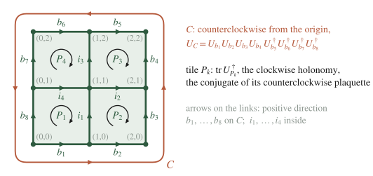
Figure 1. The 2×2 loop and its tiling. Arrows mark the positive direction of each link; the loop runs along b1, b2, b3, b4 and against b5, b6, b7, b8, and each tile carries the conjugate of its counterclockwise plaquette.

The expectation value is

$$⟨W_F(C)⟩=\frac{1}{Z}\int \prod _{\ell }d{U}_{\ell }\frac{1}{N}\mathrm{tr}{U}_C\prod _P{a}_0[1+\sum _{r\ne 0}{d}_r{\tilde{c}}_r{\chi }_r(U_P)],$$

and the factors $a_0$ cancel against Z. Expanding the product over plaquettes, each term picks for every plaquette either 1 or one term $d_r{\tilde{c}}_r{\chi }_r(U_P)$. By (G0) a link that appears once gives zero, so each boundary link must be met by a plaquette that contains it. The cheapest way is to pick, on the four plaquettes inside C, the conjugate fundamental ${\chi }_{\bar{F}}(U_P)=\mathrm{tr}{U}_P^{†}$, with weight $d_{\bar{F}}{\tilde{c}}_{\bar{F}}=N{\tilde{c}}_F$ (for SU(2), ${\chi }_{1/2}(U_P)$ with weight $2{\tilde{c}}_{1/2}$, and $\mathrm{tr}{U}_P=\mathrm{tr}{U}_P^{†}$). The counterclockwise plaquettes, read from their lower-left corners, are

$$U_{P_1}=U_{b_1}{U}_{i_1}{U}_{i_4}^{†}{U}_{b_8}^{†},U_{P_2}=U_{b_2}{U}_{b_3}{U}_{i_2}^{†}{U}_{i_1}^{†},U_{P_3}=U_{i_2}{U}_{b_4}{U}_{b_5}^{†}{U}_{i_3}^{†},U_{P_4}=U_{i_4}{U}_{i_3}{U}_{b_6}^{†}{U}_{b_7}^{†},$$

and the term to evaluate is

$$T=\frac{1}{N}(N{\tilde{c}}_F{)}^4\int \prod _{\ell }d{U}_{\ell }\mathrm{tr}{U}_C\mathrm{tr}{U}_{P_1}^{†}\mathrm{tr}{U}_{P_2}^{†}\mathrm{tr}{U}_{P_3}^{†}\mathrm{tr}{U}_{P_4}^{†}.$$

Step 1, link $i_1$. It occurs in $\mathrm{tr}{U}_{P_1}^{†}=\mathrm{tr}(U_{b_1}^{†}{U}_{b_8}{U}_{i_4}{U}_{i_1}^{†})$ and in $\mathrm{tr}{U}_{P_2}^{†}=\mathrm{tr}(U_{i_1}{U}_{i_2}{U}_{b_3}^{†}{U}_{b_2}^{†})$, in opposite directions, and (G1) fuses the two traces:

$$\int d{U}_{i_1}\mathrm{tr}{U}_{P_1}^{†}\mathrm{tr}{U}_{P_2}^{†}=\frac{1}{N}\mathrm{tr}\left(U_{b_1}^{†}{U}_{b_8}{U}_{i_4}{U}_{i_2}{U}_{b_3}^{†}{U}_{b_2}^{†}\right),$$

the clockwise holonomy of the lower 2×1 rectangle.

Step 2, link $i_2$. The fused trace contains $U_{i_2}$, and $\mathrm{tr}{U}_{P_3}^{†}=\mathrm{tr}(U_{i_3}{U}_{b_5}{U}_{b_4}^{†}{U}_{i_2}^{†})$ contains $U_{i_2}^{†}$; (G1) gives

$$\frac{1}{N^2}\mathrm{tr}\left(U_{b_3}^{†}{U}_{b_2}^{†}{U}_{b_1}^{†}{U}_{b_8}{U}_{i_4}{U}_{i_3}{U}_{b_5}{U}_{b_4}^{†}\right),$$

the clockwise holonomy of the L-shaped region $P_1\cup P_2\cup P_3$.

Step 3, link $i_3$. With $\mathrm{tr}{U}_{P_4}^{†}=\mathrm{tr}(U_{i_3}^{†}{U}_{i_4}^{†}{U}_{b_7}{U}_{b_6})$, (G1) gives

$$\frac{1}{N^3}\mathrm{tr}\left(U_{b_5}{U}_{b_4}^{†}{U}_{b_3}^{†}{U}_{b_2}^{†}{U}_{b_1}^{†}{U}_{b_8}{U}_{i_4}{U}_{i_4}^{†}{U}_{b_7}{U}_{b_6}\right).$$

Step 4, link $i_4$. It now appears as $U_{i_4}{U}_{i_4}^{†}=1$ and drops out with no factor. The path has reached the central site (1,1) along $i_4$ and returned at once: the index loop closed around that interior site gives back the N that a fourth integral would have cost. What remains is $N^{-3}\mathrm{tr}{U}_C^{†}$, with $U_C^{†}$ the clockwise holonomy of the boundary.

Step 5, the boundary. Writing $U_C=U_{b_1}R$, (G1) on $b_1$ turns $\int \mathrm{tr}{U}_C\mathrm{tr}{U}_C^{†}$ into $\frac{1}{N}\mathrm{tr}(R{R}^{†})=\frac{1}{N}\mathrm{tr}1=1$, after which the other seven boundary links appear only in $R{R}^{†}$.

Collecting the factors,

$$T=\frac{1}{N}(N{\tilde{c}}_F{)}^4\cdot \frac{1}{N^3}\cdot 1={\tilde{c}}_F^4.$$

Every other nonvanishing term has more plaquettes, and the vacuum terms, closed surfaces starting with the six faces of a cube at order ${\tilde{c}}^6$, cancel between numerator and denominator except where they touch the tiling (§4.3). Therefore $⟨W_F(C_{2\times 2})⟩={\tilde{c}}_F^4[1+O({\tilde{c}}_F^4)]$. The bare integral, $N^{-3}$, was also checked by Monte Carlo sampling of the Haar measure for SU(2) and SU(3).

4.2 Every disk weighs the same: the tiling rule [Computed for disks; other topologies Sketched and checked.]

The counting of §4.1 generalizes. Let Σ be a surface of $|\Sigma |$ plaquettes bounded by C, embedded (each link of Σ belongs to exactly two of its plaquettes, or to one plaquette and the loop) and oriented so that every link is traversed once in each direction. Each tile contributes $N{\tilde{c}}_F$ times a trace; each link integral, interior or on C, costs $1/N$ by (G1) or (G2); and after all integrations every site of Σ, interior or on C, closes one index loop and gives a factor N, as the central site did in Step 4 and the boundary sites did in Step 5. With V sites, E links and $F=|\Sigma |$ plaquettes the term is

$$\frac{1}{N}(N{\tilde{c}}_F{)}^F{N}^{-E}{N}^V={\tilde{c}}_F^{|\Sigma |}{N}^{\chi (\Sigma )-1},\chi =V-E+F,$$

where χ is the Euler characteristic. For a disk $\chi =1$, and the term is exactly ${\tilde{c}}_F^{|\Sigma |}$, with no dependence on N or on the shape. The same counting with b boundary loops, each normalized by $1/N$, gives ${\tilde{c}}_F^{|\Sigma |}{N}^{\chi -b}$: a sphere without boundary, such as the surface of a cube, gives $N^2{\tilde{c}}_F^6$ for each orientation, and an annulus between two loops gives $N^{-2}{\tilde{c}}_F^{|\Sigma |}$ (used in §7.6). These values were checked against Monte Carlo evaluations of the bare Haar integrals for the 1×2 and 2×2 disks, the decorated disk of §4.3, the cube and the annulus of §7.6, for SU(2) and SU(3). For a representation r the same argument, with Schur’s formula for $D^r$, gives ${\tilde{c}}_r^{|\Sigma |}$ for a disk.

The dominant surface is the one of smallest area. For a planar loop it is unique, the flat tiling of area $A(C)$, and

$$\boxed{⟨W_F(C)⟩={\tilde{c}}_F^{A(C)}[1+O({\tilde{c}}_F^4)],\sigma =-\ln {\tilde{c}}_F.}$$

For the $R\times T$ rectangle, $V(R)=-{\lim }_{T\to \infty }{T}^{-1}\ln ⟨W⟩=\sigma R$: a linear potential, in lattice units, for every compact group. At small β, $\sigma \simeq \ln (2/\beta )$ for U(1), $\ln (4/\beta )$ for SU(2) and $\ln (2N^2/\beta )$ for SU(N ≥ 3); at $\beta =1$ the leading values are $0.807$, $1.426$ and, for SU(3), $2.81$.

Physical picture. The selection rules are Gauss’s law for the electric flux emitted by the static sources. Flux cannot end on a link, so the sheet of plaquettes that carries it must be a surface bounded by the loop, and each unit of area costs a factor ${\tilde{c}}_F$: the string tension is the free energy per unit area of the flux sheet. At strong coupling the sheet is rigid and flat, and nothing in the calculation used the group being abelian, which is why confinement at small β is universal. The statement concerns the lattice theory at large lattice spacing; what the sheet does at larger β, and what survives in the continuum, are §§7.3–7.4.

4.3 The first correction: decorated surfaces [Controlled to O(c̃⁴).]

The cheapest surfaces after the flat one are obtained by removing one plaquette p of the minimal surface and replacing it by the other five faces of a unit cube that has p as a face (Figure 2a). The result is again an embedded disk, now with $A+4$ plaquettes, so by §4.2 it contributes ${\tilde{c}}_F^{A+4}$ with group factor 1 (the bare integral for the decorated 1×1 loop, $N^{-4}$, was checked for SU(2) and SU(3)). There are A choices of p, and the cube can stand on either side of the plane in each of the $d-2$ transverse directions, $2(d-2)$ choices.

For SU(3), and likewise for ${\mathbb{Z}}_3$, a second configuration enters one order later. Keep p in the sheet but let it carry the conjugate representation, and attach the same five-face box with the orientation that runs along $\partial p$ in the same direction as the sheet. On each edge of p three fundamental lines then meet in the same direction, which the ε-tensor of SU(3) allows: $3\otimes 3\otimes 3$ contains one singlet, so $\int dU(\mathrm{tr}U{)}^3=1$. The box fuses to $N^{-4}\mathrm{tr}{U}_{\partial p}$, the bare integral is $N^{-4}\int dU(\mathrm{tr}U{)}^3=1/81$, and the weight relative to the flat sheet is $(3{\tilde{c}}_F{)}^5/81=3{\tilde{c}}_F^5$ per location, with the same $2(d-2)A$ locations. For U(1), ${\mathbb{Z}}_2$, SU(2) and SU($N\ge 4$) the integral $\int (\mathrm{tr}U{)}^3$ vanishes and the configuration does not contribute (the SU(N) analogue needs N lines on an edge and appears only at much higher order).

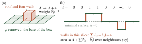
Figure 2. (a) A decorated surface: one plaquette p of the minimal sheet is replaced by the other five faces of a unit cube, adding four plaquettes. (b) A slice of the sheet in the solid-on-solid picture of §7.3: an integer height h on each plaquette of the minimal surface, and one wall plaquette for every unit step between neighbours.

Vacuum bubbles cancel between numerator and denominator, apart from configurations that overlap the sheet: for the groups without a cubic invariant, a cube that shares a plaquette or a link with it changes $\ln ⟨W⟩$ at relative order ${\tilde{c}}^6$ (for SU(3), the ε-tensor box above is exactly such an overlap, at order ${\tilde{c}}^5$). Two decorations appear $\frac{1}{2}[2(d-2)A{]}^2$ times at order ${\tilde{c}}^8$, minus $O(A)$ overlapping pairs, which is the square of the single-decoration term up to $O(A{\tilde{c}}^8)$. The series exponentiates, and

$$⟨W_F(C)⟩={\tilde{c}}_F^A\exp [2(d-2)A{\tilde{c}}_F^4+O(A{\tilde{c}}_F^6)],\boxed{\sigma =-\ln {\tilde{c}}_F-2(d-2){\tilde{c}}_F^4+O({\tilde{c}}_F^6)}$$

for U(1), ${\mathbb{Z}}_2$, SU(2) and SU($N\ge 4$), while for SU(3) the ε-tensor boxes add one term,

$${\sigma }_{SU(3)}=-\ln {\tilde{c}}_F-2(d-2){\tilde{c}}_F^4-6(d-2){\tilde{c}}_F^5+O({\tilde{c}}_F^6),$$

which in $d=4$ is the familiar $-\ln u-4u^4-12u^5$ of the SU(3) strong-coupling series. At this order the decorations shift only the area term: every plaquette of the sheet can carry one, so their number is exactly $2(d-2)A$. Perimeter terms first appear at order ${\tilde{c}}^6$, for instance from boxes on a base of two adjacent plaquettes, whose number $2(d-2)(2A-R-T)$ for an $R\times T$ loop has an area part and a perimeter part. For SU(2) in $d=4$ at $\beta =1$, $\sigma =1.426-0.013=1.413$, a one per cent correction; for U(1) at the same β, where ${\tilde{c}}_1=0.446$ is larger, the correction is $0.159$ out of $0.807$. The decorations are Wilson’s unit cubes attached to the minimal surface (§9) and Kogut’s “house” (RMP 55, §IV.A), where $d=3$ gives $\sigma =-\ln \tanh \beta -2{\tanh }^4\beta$ for ${\mathbb{Z}}_2$.

5. The continuum limit and the normalization of β [Controlled to O(a²).]

5.1 U(1)

Take a smooth gauge field A and put $a_{\mu }(x)={\int }_{{\ell }_{\mu }(x)}A$, writing a for $a_{\mathrm{lat}}$ in this section. By Stokes, $(da{)}_P={\oint }_{\partial P}A={\int }_{P}F$, and the midpoint rule ${\int }_{-a/2}^{a/2}{\int }_{-a/2}^{a/2}f=a^{2}f(0)+\frac{a^4}{24}({\partial }_1^2+{\partial }_2^2)f(0)+O(a^6)$ (the odd terms vanish by symmetry, and ${\int }_{-a/2}^{a/2}{t}^{2}dt=a^3/12$) gives, about the center $x_P$ of the plaquette,

$$(da{)}_P=a^2{F}_{\mu \nu }(x_P)+\frac{a^4}{24}({\partial }_{\mu }^2+{\partial }_{\nu }^2)F_{\mu \nu }(x_P)+O(a^6).$$

Then $1-\cos (da{)}_P=\frac{1}{2}(da{)}_P^2-\frac{1}{24}(da{)}_P^4+\dots$, and with ${\sum }_P={\sum }_x{\sum }_{\mu <\nu }$ and $a^d{\sum }_{x}f(x_P)\to \int d^{d}xf$ (for a smooth, decaying f the error of this midpoint sum vanishes faster than any power of a),

$$S=\frac{\beta a^{4-d}}{2}\int d^{d}x\sum _{\mu <\nu }{F}_{\mu \nu }^2[1+O(a^2)]=\frac{\beta a^{4-d}}{4}\int d^{d}x{F}_{\mu \nu }{F}_{\mu \nu }[1+O(a^2)].$$

Matching $\frac{1}{4e^2}\int F_{\mu \nu }{F}_{\mu \nu }$ of conventions §4 gives

$$\boxed{\beta =\frac{1}{e^2{a}^{4-d}}(\text{U}(1)),}$$

with $e^2$ of mass dimension $4-d$. The corrections are $\frac{a^2}{24e^2}\int {\sum }_{\mu <\nu }{F}_{\mu \nu }({\partial }_{\mu }^2+{\partial }_{\nu }^2)F_{\mu \nu }$, of dimension six, and $-\frac{a^4}{24e^2}\int {\sum }_{\mu <\nu }{F}_{\mu \nu }^4$, of dimension eight; for the canonical field $A=e{A}_c$ they are suppressed by $a^2$ and by $e^2{a}^4$. A numerical check on a smooth field confirms that the relative error of the expansion of $(da{)}_P$ drops from $O(a^2)$ to $O(a^4)$ once the $a^4/24$ term is kept.

5.2 SU(N)

With $U_{\ell }=\mathcal{P}\exp (i{\int }_{\ell }A)$, $A=A^a{T}^a$ and $\mathrm{tr}{T}^a{T}^b=\frac{1}{2}{\delta }^{ab}$, write each link as $U_{\mu }(x)=\exp [ia{A}_{\mu }(x+\frac{a}{2}\hat{\mu })+O(a^3)]$ and combine the four factors of $U_P$ with $e^X{e}^Y=e^{X+Y+\frac{1}{2}[X,Y]+\dots }$. The abelian parts add up to $i{a}^2({\partial }_{\mu }{A}_{\nu }-{\partial }_{\nu }{A}_{\mu })$, and the group commutator $e^{ia{A}_{\mu }}{e}^{ia{A}_{\nu }}{e}^{-ia{A}_{\mu }}{e}^{-ia{A}_{\nu }}=e^{-a^2[A_{\mu },A_{\nu }]+O(a^3)}$ supplies the rest, so that

$$U_P=\exp \{i{a}^2{F}_{\mu \nu }+O(a^3)\},F_{\mu \nu }={\partial }_{\mu }{A}_{\nu }-{\partial }_{\nu }{A}_{\mu }+i[A_{\mu },A_{\nu }].$$

Write $U_P=e^{i{X}_P}$ with $X_P$ hermitian. Then $\mathrm{Re}\mathrm{tr}(1-U_P)=\mathrm{tr}(1-\cos X_P)=\frac{1}{2}\mathrm{tr}{X}_P^2-\frac{1}{24}\mathrm{tr}{X}_P^4+\dots$, and

$$\mathrm{tr}{X}_P^2=a^4\mathrm{tr}{F}_{\mu \nu }(x_P{)}^2+O(a^6),$$

with no $O(a^5)$ term. Such a term would be built from $A_{\mu }$, $A_{\nu }$ and their in-plane derivatives with an odd number of in-plane indices, so it would change sign under the rotation by π about $x_P$ in the $(\mu ,\nu )$ plane; that rotation maps the plaquette onto itself with its orientation, and $\mathrm{tr}{X}_P^2$, a class function of $U_P$, is invariant under it. [Checked numerically for a smooth SU(2) field: $\mathrm{Re}\mathrm{tr}(1-U_P)/\left(\frac{a^4}{2}\mathrm{tr}{F}^2\right)-1$ is $-0.043$, $-0.011$ and $-0.0028$ at $a=0.2,0.1,0.05$, and fails to converge if the sign of the commutator in F is reversed.] Summing over plaquettes,

$$S=\frac{\beta }{N}\sum _P\mathrm{Re}\mathrm{tr}(1-U_P)=\frac{\beta a^{4-d}}{2N}\int d^{d}x\sum _{\mu <\nu }\mathrm{tr}{F}_{\mu \nu }^2[1+O(a^2)]=\frac{\beta a^{4-d}}{4N}\int d^{d}x\mathrm{tr}{F}_{\mu \nu }{F}_{\mu \nu }[1+O(a^2)],$$

and matching $\frac{1}{2g^2}\int \mathrm{tr}{F}_{\mu \nu }{F}_{\mu \nu }=\frac{1}{4g^2}\int F_{\mu \nu }^a{F}_{\mu \nu }^a$ of conventions §4 gives

$$\boxed{\beta =\frac{2N}{g^2{a}^{4-d}}(\text{SU}(N)),\text{that is,}\beta =\frac{2N}{g^2}\text{ in }d=4.}$$

The factor 2N is specific to SU(N): it comes from $\mathrm{tr}{T}^a{T}^b=\frac{1}{2}{\delta }^{ab}$ and the $1/N$ in front of the action. The U(1) link $e^{ia}$ is generated by the number 1, whose square is 1; setting $N=1$ in the SU(N) formula, $\beta =2/e^2$, would produce $\frac{1}{2e^2}\int F_{\mu \nu }{F}_{\mu \nu }$, twice the Maxwell action of the conventions, that is, a unit Wilson line of charge $e/\sqrt{2}$; this is why the two formulas are never interchanged.

5.3 What the classical limit shows

The expansion above is classical: it shows that Wilson’s action reproduces the continuum action on smooth fields, with irrelevant corrections. In the quantum theory the typical plaquette angle at weak coupling is of order ${\beta }^{-1/2}$, so the expansion in $X_P$ is the weak-coupling expansion, and the continuum limit is taken by sending $a\to 0$ with β adjusted to keep physical quantities fixed. In $d=3$ this means $\beta =1/(e^{2}a)\to \infty$ at fixed $e^2$. In $d=4$ it means $\beta \to \infty$ for SU(N), by asymptotic freedom (§7.4), and a finite β inside the Coulomb phase for U(1) (Week 11). Either way, the strong-coupling results of §4 describe the lattice theory at large lattice spacing, where the irrelevant terms are as large as the leading one.

6. Creutz ratios and the handoff to Monte Carlo [Computed.]

The rectangular loop contains more than the area term. The self-energy of the static sources gives a term proportional to the perimeter (in the continuum it diverges like $1/a$), and the corners give a constant. At any coupling we may write

$$-\ln ⟨W(I,J)⟩=\sigma IJ+f(I)+g(J)+ϵ(I,J),$$

where f and g collect everything that depends on one side only (perimeter, corners, constants) and ε is the rest, for instance a Coulomb-like term. Creutz’s ratio (he wrote χ; we write R to keep χ for characters),

$$R(I,J)=-\ln \frac{⟨W(I,J)⟩⟨W(I-1,J-1)⟩}{⟨W(I,J-1)⟩⟨W(I-1,J)⟩},$$

removes f and g exactly, since $f(I)+f(I-1)-f(I)-f(I-1)=0$ and likewise for g. The area terms combine to $\sigma [IJ+(I-1)(J-1)-I(J-1)-(I-1)J]=\sigma$, so that

$$R(I,J)=\sigma +[ϵ(I,J)+ϵ(I-1,J-1)-ϵ(I,J-1)-ϵ(I-1,J)],$$

where the bracket is a mixed second difference of ε, which falls off for large loops (for $ϵ=-\alpha J/I$ it is $\alpha /I(I-1)$). At strong coupling, with $W(I,0)=W(0,J)=1$, §§4.2–4.3 give $R(I,J)=-\ln {\tilde{c}}_F-2(d-2){\tilde{c}}_F^4+O({\tilde{c}}_F^6)$ for all $I,J\ge 1$ (with $-6(d-2){\tilde{c}}_F^5$ added for SU(3)); at higher orders the numbers of excitations take the form $aIJ+bI+cJ+e$ once the loop is large enough to contain them, so R isolates the area coefficient order by order. Creutz used these ratios in the first Monte Carlo study of SU(2) and found them crossing over, at intermediate β, from the strong-coupling behaviour to the scaling expected from asymptotic freedom [Stated — refs: Creutz, PRD 21 (1980) 2308]: numerical evidence that no phase transition separates the two regimes in $d=4$. The course leaves the numerical route here; its later weeks use the lattice for exact dualities and phase structure.

7. Subtleties and fine print

7.1 Gauge covariance, base points and the real part. Only class functions of closed holonomies are observable (§1.2). This is why the plaquette enters the action through a character, why the action takes the real part (plaquettes are unoriented), and why the continuum field strength appears only through $\mathrm{tr}{F}^2$: $F_{\mu \nu }$ transforms by conjugation, like $U_P$, and for $N\ge 2$ neither is invariant. For U(1), $U_P$ and F are invariant, a special feature of the abelian group.

7.2 Gauge fixing is allowed and never needed [Proved.] The gauge group of the lattice theory is a product of one copy of G per site, compact, with total Haar volume 1, so the integral over link variables is finite without gauge fixing and no Faddeev–Popov procedure is required; this is what Wilson meant by treating the gauge fields as angular variables. Gauge fixing is nevertheless allowed. Choose a maximal tree T, a set of links that contains no closed loop and reaches every site. For fixed tree links there is a unique gauge transformation with $g=1$ at a root site that sets them to 1: move out from the root along the tree with $g_{x+\hat{\mu }}=g_x{U}_{\mu }(x)$. For a gauge-invariant f, write $\int {\prod }_{\ell }d{U}_{\ell }f=\int {\prod }_{\ell \in T}d{U}_{\ell }\int {\prod }_{\ell \notin T}d{U}_{\ell }f(U)$. In the inner integral replace $f(U)$ by $f(U^g)$ with the tree-trivializing g. Since g depends only on the tree links, $U_{\ell }\to g_x{U}_{\ell }{g}_y^{-1}$ is, for each link off the tree, a left and a right multiplication by fixed elements, which preserves the Haar measure. The inner integral therefore equals its value at $U_T=1$, independently of the tree links, and the outer integral gives 1:

$$\int \prod _{\ell }d{U}_{\ell }f(U)=\int \prod _{\ell \notin T}d{U}_{\ell }f(U){|}_{U_{\ell }=1,\ell \in T}.$$

The axial gauge is the case of a comb-shaped tree. The Jacobian is 1, and no gauge-invariant quantity changes; in $d=2$ with open boundaries the remaining links correspond one to one to the plaquettes, and Problem 4 turns this into an exact solution.

7.3 The radius of convergence and roughening.

What converges. The logarithm of Z per site and the string tension $\sigma (\beta )$ are given at small β by convergent expansions in the coefficients ${\tilde{c}}_r$: the number of connected surfaces of n plaquettes grows at most exponentially in n, and each weighs ${\tilde{c}}^n$ times a bounded group factor. Osterwalder and Seiler proved the convergence, and the area law at small β, for every compact gauge group [Stated — refs: Osterwalder–Seiler 1978; Kogut RMP 55 §IV.A].

The sheet as a height model. In the regime of §4.3 the relevant surfaces are the flat sheet with bumps. Neglecting overhangs and closed bubbles (the solid-on-solid approximation), a surface over the minimal one in $d=3$ is described by an integer height $h_x$ on each plaquette x of the minimal surface, with $h=0$ outside the loop, and its area is $A+{\sum }_{⟨xy⟩}|h_x-h_y|$, one wall plaquette per unit step between neighbouring columns (Figure 2b). Every such surface is an embedded disk, so by §4.2 it weighs ${\tilde{c}}_F$ to the power of its area, and

$$⟨W_F(C)⟩\simeq {\tilde{c}}_F^A{Z}_{\mathrm{SOS}},Z_{\mathrm{SOS}}=\sum _{\{h\}}\exp (-K\sum _{⟨xy⟩}|h_x-h_y|),K=-\ln {\tilde{c}}_F,$$

the absolute-value solid-on-solid model at coupling K. Its lowest excitation, $h_x=\pm 1$ on one site, has four steps and weight $2{\tilde{c}}_F^4$ per site: the decorations of §4.3 in $d=3$. In $d=4$ the height becomes a two-component transverse displacement.

Roughening. At large K (small β) the surface is smooth, its height fluctuations are bounded, and the expansion in $e^{-K}$ converges. At a finite coupling $K_R$ it roughens: the height fluctuations grow logarithmically with the size of the surface, and its free energy has an essential singularity of the form $\exp (-B/\sqrt{T-T_R})$ at the transition [Stated — refs: Kogut RMP 55 §V.C]. This is the transition of the height model of Week 3 §3, which by Poisson duality is the BKT transition of the XY model seen from the height side (Chui–Weeks), now appearing on the confining string. For the gauge theory it means that $\sigma (\beta )$ is non-analytic at a roughening coupling ${\beta }_R$, and that the strong-coupling expansions have a radius of convergence bounded by the roughening point [Stated — refs: Kogut RMP 55 §V.C and the papers cited there].

What roughening changes. It is a transition of the flux sheet alone, visible only in large Wilson loops; the bulk free energy is analytic there, and σ stays positive on both sides, so confinement persists. What changes is the geometry of the flux tube. In the rough phase its mean-square width grows logarithmically with its length, its transverse fluctuations are massless and add the universal term $-\frac{(d-2)\pi }{24R}$ to the potential [Stated — refs: Kogut RMP 55 §V.B], and the rotational symmetry of the static potential is restored at long distances (§V.C there). In the 3d ${\mathbb{Z}}_2$ gauge theory, whose flux sheet is the interface of the dual Ising model of Week 5, the interface roughens at $T_R\approx \frac{1}{2}{T}_c$ of the Ising model, deep inside the confining region of the gauge theory [Stated — refs: Kogut RMP 55 §V.C, Fig. 40].

7.4 Why strong coupling cannot see asymptotic freedom. For SU(N) in $d=4$, asymptotic freedom puts the continuum limit at $g\to 0$, that is $\beta \to \infty$, where the lattice spacing in physical units vanishes as $a\Lambda \propto e^{-1/(2b_0{g}^2)}$ with $b_0=11N/48{\pi }^2$ at one loop [Stated — refs: Kogut RMP 51 §VIII.B; Kogut RMP 55 §§II.A, IV.D]. With $g^2=2N/\beta$ this reads

$$\sigma a^2\propto (a\Lambda {)}^2\propto \exp (-\frac{\beta }{2N{b}_0})=\exp (-\frac{24{\pi }^2}{11N^2}\beta ),$$

which is $e^{-8{\pi }^2\beta /33}$ for SU(3). Three facts keep the strong-coupling series away from this regime. The series is defined near $\beta =0$ and has a finite radius, bounded by the roughening point (§7.3), so it cannot be continued to large β. Its truncations decrease only logarithmically, $\sigma \simeq \ln (2N^2/\beta )$, where the continuum limit requires an exponential decrease. And inside its domain σ is of order one or larger in lattice units, so correlation lengths are at most a lattice spacing and rotational invariance is broken: there is no continuum physics there to see. What strong coupling does establish is that the lattice theory confines at small β for every compact group. The continuum statement needs in addition the absence of a phase transition between small and large β, which Monte Carlo supports for SU(N) (§6) and nobody has proved.

7.5 Representation dependence and a preview of N-ality. The leading term $⟨W_r(C)⟩={\tilde{c}}_r^A$ is the first term for a loop of fixed size as $\beta \to 0$, and for higher representations it fails to describe large loops. The adjoint of SU(N) is contained in $F\otimes \bar{F}$, so a closed tube of fundamental plaquettes running along C, with C drawn on its surface (Figure 3), is allowed by the selection rules: at each link of C the adjoint of the loop and the F and $\bar{F}$ of the two tube plaquettes that contain the link combine into the singlet, once. The smallest such tube is the surface of the ring of $2(R+T)-4$ unit cubes that lines the inside of an $R\times T$ loop; each cube of the ring exposes four faces, so the tube has $4P-16$ plaquettes, with $P=2(R+T)$. It gives a perimeter law $\propto {\tilde{c}}_F^{4P-16}$, while the adjoint sheet gives ${\tilde{c}}_{\mathrm{adj}}^A\sim {\tilde{c}}_F^{2A}$ (§3.5), and for large loops the tube wins. The adjoint charge is screened by gluons, and at leading logarithmic order the crossover sits where $2A\simeq 4P-16$, at square loops of side about 7 [Sketched; the group factor of the tube is Problem 5⋆].

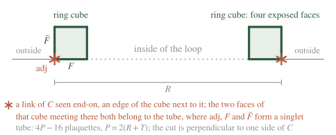
Figure 3. The tube that screens the adjoint loop, in cross-section. A ring of unit cubes lines the inside of the loop; its surface is a torus of fundamental plaquettes that passes through every link of C (marked *), where the adjoint combines with F and F̄ into a singlet.

The general mechanism is the center. The element $z=e^{2\pi i/N}$ acts on a representation with $k_r$ boxes (mod N) as $z^{k_r}$, its N-ality, and the selection rule of §2.3 says that sheets of plaquettes may change representation along the way while their N-ality stays fixed. Gluons, of N-ality 0, can therefore screen any representation down to the lightest one of the same N-ality, and loops of N-ality 0 obey a perimeter law at large size. This is the local form of the electric ${\mathbb{Z}}_N$ 1-form (center) symmetry of pure SU(N) gauge theory, under which Wilson lines carry the charge $k_r$; the area law of the fundamental loop says that this symmetry is unbroken (conventions §6, higher-form-symmetries; Week 14 and Semester II Block 1). For U(1) the electric 1-form symmetry is U(1) itself, there are no charged gauge bosons, and every charge is conserved; even so, the flat sheet of charge 2 is not the cheapest surface for a large loop in $d\ge 3$ (Problem 9⋆⋆). Finally, Casimir scaling of the leading coefficient depends on the action: it holds for the heat-kernel action (Problem 6⋆) and in the Hamiltonian strong-coupling limit of Week 7, where $\sigma =\frac{g^2}{2}{C}_2(F)$ (conventions §4), and it fails for the Wilson action (§3.5).

7.6 The Polyakov line at finite temperature. Make Euclidean time periodic with $N_{\tau }$ sites, so that $T=1/(N_{\tau }a)$, and define the Polyakov loop $L(\vec{x})=\frac{1}{N}\mathrm{tr}{\prod }_{t=0}^{N_{\tau }-1}{U}_0(\vec{x},t)$ (often written P; we keep P for plaquettes). Multiply every time-like link on one time slice by $z=e^{2\pi i/N}$. Each plaquette that contains one of these links contains exactly one more, traversed in the opposite direction, so the action is invariant, while $L\to zL$. Therefore $⟨L⟩=z⟨L⟩$ vanishes unless this center symmetry is broken spontaneously. Every term of the strong-coupling expansion obeys the selection rule, so $⟨L⟩=0$ order by order: the expansion cannot show $⟨L⟩\ne 0$, and the deconfinement transition at high temperature lies outside its radius of convergence. The correlator is computable. For $\vec{x}$ and $\vec{y}$ at distance r along an axis, the strip of $N_{\tau }r$ time-like plaquettes between the two lines is an annulus bounded by the two loops (tiles oriented against the lines), and §4.2 gives

$$⟨L(\vec{x})L(\vec{y}{)}^{†}⟩=\frac{1}{N^2}{\tilde{c}}_F^{N_{\tau }r}[1+\dots ]$$

(without the $1/N^2$ for U(1)), so the free energy of a static pair, $F_{q\bar{q}}(r)=-T\ln ⟨L{L}^{†}⟩=\sigma r+2T\ln N$ in lattice units ($T{N}_{\tau }=1$), rises linearly with the zero-temperature tension. As $N_{\tau }$ decreases, the effective coupling between neighbouring Polyakov lines, ${\tilde{c}}_F^{N_{\tau }}$ at leading order, grows until the center symmetry breaks: this is deconfinement, whose universality class, when the transition is continuous, is that of a ${\mathbb{Z}}_N$ spin model in $d-1$ dimensions [Stated — refs: Svetitsky–Yaffe 1982]. Week 14 returns to it.

7.7 Phase structure by group and dimension. Figure 4 collects what is known and what is expected. In $d=2$ the tiling is exact for every group (Problem 4): an area law at every β, and no roughening, since the sheet has no transverse direction. In $d=3$ compact U(1) confines at every coupling, at weak coupling through Polyakov’s monopole plasma (Week 9 and Week 10, on the dual variables of Week 8) and for the Villain action at all couplings by a theorem [Stated — refs: Göpfert–Mack 1982]; in the language of conventions §6, its electric $U(1{)}^{(1)}$ symmetry is unbroken at every coupling. In $d=4$ compact U(1) has a Coulomb phase at large β, with a massless photon and a perimeter law, in which the electric 1-form symmetry is spontaneously broken [Stated — refs: Guth 1980 for the Villain action; Fröhlich–Spencer 1982]; a transition separates it from the confined phase. For SU(N) in $d=4$ no bulk transition is expected between the strong-coupling region and the continuum limit at $\beta \to \infty$, on the evidence of Monte Carlo, and the only non-analyticity expected along the way at zero temperature is the roughening of the flux sheet.

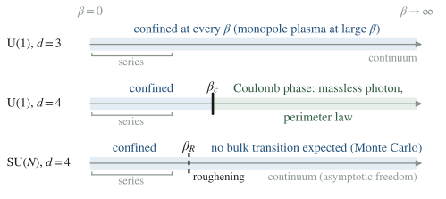
Figure 4. Phase structure in β at zero temperature. “Series” marks the small-β region where the strong-coupling expansion converges; ${\beta }_R$ is the roughening of the flux sheet (§7.3), a transition of the string that leaves the bulk analytic, drawn only for SU(N), where §7.3 cites it; ${\beta }_c$ is the transition of 4d compact U(1). Positions along the β axes are schematic.

8. Common misconceptions

• “The strong-coupling area law proves that QCD confines.” It is tempting because the area law at small β is a theorem, and it holds for SU(3). The theorem concerns the lattice theory at large lattice spacing. The continuum limit of SU(N) in $d=4$ is at $\beta \to \infty$, beyond the radius of convergence (§§7.3–7.4), and the same computation gives an area law for 4d compact U(1), whose continuum limit is Maxwell theory with a Coulomb potential. Confinement in the continuum requires in addition that no phase transition intervene, which Monte Carlo supports for SU(N) and nobody has proved.
• “The Haar measure needs gauge fixing, as the continuum path integral does.” The continuum intuition comes from gauge orbits of infinite volume. On the lattice the orbits are compact, of volume 1 per site, and the unfixed integral is finite; gauge fixing on a maximal tree is allowed, with unit Jacobian (§7.2), and changes no gauge-invariant quantity.
• “SU(2) and U(1) are the cases N = 2 and N = 1 of the SU(N) formulas.” The actions look alike, and the groups differ exactly where it matters. The SU(2) fundamental is pseudo-real, so ${\tilde{c}}_{1/2}\simeq \beta /4$, twice $\beta /2N^2$ at $N=2$ (§3.3); ${\mathbb{Z}}_2$, whose charge is real, shows the same doubling against ${\mathbb{Z}}_{N\ge 3}$ (Problem 3). The U(1) charge normalization fixes $\beta =1/e^2$ in $d=4$, and $\beta =2N/g^2$ at $N=1$ would double the Maxwell term (§5.2).
• “At strong coupling, string tensions obey Casimir scaling.” Casimir scaling is seen in simulations at intermediate distances and holds in the Hamiltonian strong-coupling limit, which makes the statement plausible. For the Wilson action the leading coefficient counts fundamental factors, ${\sigma }_1/{\sigma }_{1/2}\to 2$ for SU(2) (§3.5); Casimir scaling of the leading coefficient belongs to the heat-kernel action (Problem 6⋆); and for large loops the tension depends only on the N-ality (§7.5).

9. Historical note

Wilson’s “Confinement of quarks” (Phys. Rev. D 10 (1974) 2445) looked for a mechanism that keeps quarks bound, modelled on Schwinger’s two-dimensional electrodynamics. Its §III formulates a gauge theory on a four-dimensional Euclidean lattice, with the gauge field on links as an angular variable, periodic with period 2π, which, in Wilson’s words, “makes a gauge-fixing term unnecessary”. The paper works out a single abelian gauge field coupled to quarks, with a cosine of the plaquette angle as the action, and treats the non-abelian case in a few lines: the link becomes a group element, the integrations become compact group integrations, and the plaquette action is written with the adjoint representation, with the remark that any representation would do. Its §IV develops the strong-coupling expansion. The gauge-field average of a closed quark path vanishes unless elementary squares fill a surface bounded by the path, so it falls exponentially with the minimal enclosed area, as $(g^2{)}^{-A}$ in lattice units; unit cubes attached to the minimal surface give about as many extra terms at the next order as the surface has plaquettes, so the expansion has to be organized for the logarithm of the loop; and the sum over surfaces has the structure of the string models of hadrons of the time. Wilson was explicit about the limits: the strong-coupling limit is far from Lorentz invariant, and for the abelian theory he expected a phase transition at intermediate coupling to a phase of massless photons and free charges. The character-expansion machinery of this week was systematized in the following years (reviewed by Drouffe and Itzykson in 1978), Osterwalder and Seiler proved the convergence of the expansion in 1978, and whether SU(N) has a transition between strong and weak coupling was taken up by Monte Carlo, starting with Creutz in 1980.

10. What to take away

1. Haar measure plus Schur’s lemma is a graphical calculus. A link integrates to zero unless its representations contain the singlet, two traces sharing a link fuse at the cost $1/N$, and the center turns this into an N-ality selection rule, which the pseudo-real SU(2) and the abelian U(1) satisfy in their own ways.
2. The character coefficients are computed. ${\tilde{c}}_n=I_n/I_0\simeq \beta /2$ for U(1), ${\tilde{c}}_{1/2}=I_2/I_1\simeq \beta /4$ for SU(2) and ${\tilde{c}}_F\simeq \beta /2N^2$ for SU(N ≥ 3); a representation first reached with $n_r$ fundamental factors has ${\tilde{c}}_r=O({\beta }^{n_r})$.
3. The area law is a tiled disk. Every embedded disk of fundamental plaquettes weighs exactly ${\tilde{c}}_F^{|\Sigma |}$, the powers of N cancelling through the Euler characteristic; therefore $⟨W_F⟩={\tilde{c}}_F^A(1+\dots )$ and $\sigma =-\ln {\tilde{c}}_F-2(d-2){\tilde{c}}_F^4+O({\tilde{c}}_F^6)$ for U(1), ${\mathbb{Z}}_2$, SU(2) and SU($N\ge 4$); for SU(3) the baryon vertex adds $-6(d-2){\tilde{c}}_F^5$.
4. The coupling is fixed by the continuum limit. Wilson’s action tends to $\frac{1}{4e^2}\int F^2$ with $\beta =1/e^2{a}^{4-d}$ for U(1) and to $\frac{1}{2g^2}\int \mathrm{tr}{F}^2$ with $\beta =2N/g^2{a}^{4-d}$ for SU(N), with $O(a^2)$ corrections; Creutz ratios remove the perimeter and corner terms exactly.
5. Strong coupling proves lattice confinement at small β, and the rest is dynamics. Roughening bounds the series, the continuum limit of SU(N) sits at $\beta \to \infty$, and the group and the dimension decide what happens in between: 3d U(1) confines at every coupling, 4d U(1) has a Coulomb phase, and 4d SU(N) is believed to confine at every coupling.

11. Looking ahead: Week 7

We have the Euclidean picture. Week 7 makes time continuous: the anisotropic lattice, its transfer matrix and the limit that yields the Kogut–Susskind Hamiltonian, with link rotors, the electric field as their conjugate, and the Gauss law as an operator constraint. The character basis of this week becomes the electric-flux basis there, the strong-coupling flux sheets become electric strings whose energy per unit length is $\frac{g^2}{2}{C}_2(r)$, and the ${\mathbb{Z}}_2$ Hamiltonian turns out to be the toric code one renaming away, planted for Semester II.

12. Problem set

Problems 1–4 are the classroom core and are solvable from the note alone; Problems 5⋆–7⋆ are self-study consolidation, each with a hint or an indicated method; Problems 8⋆⋆ and 9⋆⋆ are research extensions that state what is known, what is explored, the sources they need and what counts as completion.

Core problems (everyone).

1. The 1×2 loop by hand. (a) For SU(N) with $N\ge 3$, label the seven links of the 1×2 rectangle and its two tiles as in Figure 1, integrate the shared link and then the boundary links with (G1) and unitarity, and show that the leading term of $⟨W_F⟩$ is ${\tilde{c}}_F^2$, accounting for every power of N. (b) Repeat with one tile reversed ($\mathrm{tr}{U}_P$ in place of $\mathrm{tr}{U}_P^{†}$) and show that the result vanishes for $N\ge 3$ and not for SU(2); explain both with §2.3. (c) Count the decorated surfaces of §4.3 on the 1×2 loop in d dimensions and show that $⟨W_{1\times 2}⟩={\tilde{c}}_F^2[1+4(d-2){\tilde{c}}_F^4+O({\tilde{c}}_F^6)]$ for SU(2) and SU($N\ge 4$), and that for SU(3) the ε-tensor boxes of §4.3 add $12(d-2){\tilde{c}}_F^5$ inside the bracket. (d) For SU(2) in $d=4$, evaluate the Creutz ratio $R(1,2)$ from $W(1,1)$, $W(1,2)$ and $W(0,J)=1$ at $\beta =1$ and $\beta =2$, and compare with σ of §4.3.

2. SU(2) class integrals and higher representations. (a) With the class measure of §2.2, compute $\int dU{\chi }_{1/2}^3{\chi }_{3/2}$ and $\int dU{\chi }_1^3$, and interpret each as a count of singlets. (b) Expand $e^{\frac{\beta }{2}{\chi }_{1/2}}$ to second and third order and obtain ${\tilde{c}}_1\simeq {\beta }^2/24$ and ${\tilde{c}}_{3/2}\simeq {\beta }^3/192$ without Bessel functions; compare with $I_3/I_1$ and $I_4/I_1$ at $\beta =0.1$ and $\beta =1$. (c) Show that $-\ln {\tilde{c}}_j/(-\ln {\tilde{c}}_{1/2})\to 2j$ as $\beta \to 0$, and find the leading correction to this limit.

3. Character coefficients of ${\mathbb{Z}}_N$. For the ${\mathbb{Z}}_N$ theory with $U_{\ell }=e^{2\pi i{k}_{\ell }/N}$ and $S_P=\beta (1-\cos (2\pi k_P/N))$: (a) show that the characters are $e^{2\pi ink/N}$, $n=0,\dots ,N-1$, and write ${\tilde{c}}_n(\beta )$ as a finite sum; (b) show that $N=2$ gives $\tanh \beta$ (Week 5), that $N=4$ gives ${\tilde{c}}_1=\tanh (\beta /2)$, and that ${\tilde{c}}_n\to I_n/I_0$ as $N\to \infty$ at fixed n; (c) show that ${\tilde{c}}_1\simeq \beta /2$ at small β for $N\ge 3$, against $\tanh \beta \simeq \beta$ for $N=2$, and relate the factor 2 to §3.3.

4. Two dimensions: the tiling is exact. On an open $L\times L$ lattice in $d=2$: (a) take as maximal tree all vertical links together with the horizontal links of the bottom row, and use §7.2 to set them to 1; (b) show that the plaquette variables are then $U_P(x,y)=U_h(x,y)U_h(x,y+1{)}^{†}$ in terms of the remaining horizontal links, that the change of variables to plaquettes preserves the Haar measure, and that the plaquettes are independent; (c) conclude that $⟨W_r(C)⟩={\tilde{c}}_r^{A(C)}$ exactly, at every β and for every loop, and evaluate it for SU(2) at $\beta =2$ for the 1×1, 1×2 and 2×2 loops; (d) explain why there is neither roughening nor a Coulomb phase in $d=2$.

Starred problems (Ph.D. expected; ambitious M.Sc. encouraged).

5⋆. The adjoint loop and its screening. (a) Show that the adjoint loop has the leading area term ${\tilde{c}}_{\mathrm{adj}}^A$, with ${\tilde{c}}_{\mathrm{adj}}\simeq {\beta }^2/4N^2(N^2-1)$ for $N\ge 3$ and ${\tilde{c}}_1\simeq {\beta }^2/24$ for SU(2). (b) Construct the tube of Figure 3 for an $R\times T$ loop with $R,T\ge 3$, show that the selection rules allow it, and verify that it has $4P-16$ plaquettes. (c) Write the contribution of the tube as ${\kappa }^P{\tilde{c}}_F^{4P-16}$ times a constant, with κ a nonzero group-theory factor per unit length that does not depend on the loop, and show that for any such κ the tube dominates the area term for large loops; find the crossover size of square loops at leading logarithmic order. (d) Explain why no such tube screens the fundamental loop of SU(N), and why nothing screens the charge-q loops of U(1). (Hint: $F\otimes \bar{F}=1\oplus \mathrm{adj}$ and $\mathrm{adj}\otimes F\otimes \bar{F}$ contains the singlet once; for (d) use the center rule of §2.3.)

6⋆. The heat-kernel action and Casimir scaling. Take as plaquette weight the heat kernel on G at time τ, $e^{-S_P(U)}={\sum }_r{d}_r{\chi }_r(U)e^{-\frac{\tau }{2}{C}_2(r)}$. (a) Show that ${\tilde{c}}_r=e^{-\tau C_2(r)/2}$ exactly, so that the leading coefficient obeys Casimir scaling at every τ, with the SU(2) ratios $8/3$ and $5$. (b) For U(1), where $C_2(n)=n^2$, use the periodic-Gaussian identity of conventions §3 to show that the heat kernel at $\tau =1/\beta$ is the Villain weight ${\sum }_n{e}^{-\frac{\beta }{2}(\varphi -2\pi n{)}^2}$ up to normalization (Week 1 §6.2). (c) Match τ to β for SU(2) at weak coupling by comparing $e^{-3\tau /8}$ with the large-β form of $I_2/I_1$ (use the asymptotic form of Week 1 §5.2), and find $\tau \simeq 4/\beta$. (d) Explain, with §7.5, why neither box counting nor Casimir scaling of the leading coefficient fixes the tension of very large loops.

7⋆. The U(1) plaquette to ninth order. For U(1) every character coefficient is positive, and a configuration of integer plaquette charges contributes whenever the charge is conserved at every link; on the infinite lattice every closed 2-chain is the boundary of an integer combination of cubes. (a) Show that $⟨W_{1\times 1}⟩=u+2(d-2)[u^5(1+u_2)-2u^7]+O(u^9)$, with $u=I_1/I_0$ and $u_2=I_2/I_0$, identifying the cube that removes the plaquette, the cube that doubles its charge, and the vacuum cubes that the plaquette excludes. (b) Show that the $O(u^9)$ term is $10(d-2)(2d-5)u^9$, from pairs of face-adjacent cubes. (c) Evaluate the series at $\beta =0.5$ in $d=3$ and $d=4$. (Hint: write numerator and denominator as sums over integer cube charges h; the terms in which h does not touch the plaquette cancel exactly.)

⋆⋆ problems (research extension; optional).

8⋆⋆. Roughening from the strong-coupling side. What is known. At strong coupling the flux sheet of the fundamental loop is, up to overhangs and bubbles, the absolute-value solid-on-solid model of §7.3 with $K=-\ln {\tilde{c}}_F$; solid-on-solid models roughen through a transition of BKT type, dual to the XY model (Week 3 §3, Chui–Weeks); for the 3d ${\mathbb{Z}}_2$ gauge theory the flux sheet is the Ising interface, which roughens at $T_R\approx \frac{1}{2}{T}_c$ (Kogut RMP 55 §V.C and the papers cited there). What is explored. How well the solid-on-solid picture locates the roughening coupling of a gauge theory. (a) Derive the solid-on-solid weights for the 3d ${\mathbb{Z}}_2$ or U(1) flux sheet, and list the configurations the model omits with the order in $\tilde{c}$ at which each first appears. (b) Estimate $K_R$ of the absolute-value model by a Monte Carlo simulation, from the logarithmic growth of the height variance with the linear size of the surface. (c) Translate $K_R$ into ${\beta }_R$ for ${\mathbb{Z}}_2$ through $\tanh {\beta }_R=e^{-K_R}$ and compare with the Ising-interface value, using the duality $\tanh \beta =e^{-2K^{\ast }}$ of conventions §4. Completion: the derivation of (a) with the list; $K_R$ with an error bar from at least three lattice sizes; and the comparison of (c), with a statement of which omitted configurations could account for the difference.

9⋆⋆. Charge-2 flux sheets in U(1). What is known. At leading order $⟨W_2(C)⟩\simeq {\tilde{c}}_2^A$ with ${\tilde{c}}_2=I_2/I_0$ (§3.2), and ${\tilde{c}}_1^2>{\tilde{c}}_2$ at every $\beta >0$, an instance of the Turán-type inequalities $I_1^2>I_0{I}_2$ for modified Bessel functions (checked numerically for these notes). What is explored. Whether the flat charge-2 sheet or two unit sheets dominate large charge-2 loops in $d\ge 3$. (a) In $d=3$, compare the flat charge-2 sheet with the configuration in which one unit of flux leaves the plane along the walls of a box of height one over the loop and closes along its lid, of weight ${\tilde{c}}_1^{2A+P}$; show that the second wins for large loops and find the crossover side of a square loop at $\beta =0.5$. (b) Using the positivity of all terms of the U(1) expansion, argue that the tension of large charge-2 loops lies below $-\ln {\tilde{c}}_2$ at small β, and estimate by how much. (c) Compare with the weak-coupling behaviour of charge-q loops in 3d compact QED (Week 10). Sources: the strong-coupling methods of Drouffe–Itzykson, Phys. Rep. 38 (1978) 133, and Week 10 for (c). Completion: (a) with the crossover size; (b) as an argument that states its assumptions about the cancellation of vacuum bubbles; (c) a paragraph built on the relevant formula of Week 10.

Self-study answer checkpoints

These checkpoints cover the core problems; starred and ⋆⋆ problems remain source-led.

1. The 1×2 loop. The decisive step is the shared link, which appears in $\mathrm{tr}{U}_{P_1}^{†}$ and $\mathrm{tr}{U}_{P_2}^{†}$ in opposite directions; (G1) fuses the two traces into $\frac{1}{N}\mathrm{tr}{U}_{P_1\cup P_2}^{†}$, and the boundary then gives $\frac{1}{N}\mathrm{tr}1=1$ as in Step 5 of §4.1. The result is $\frac{1}{N}(N{\tilde{c}}_F{)}^2\cdot \frac{1}{N}={\tilde{c}}_F^2$, in agreement with the Euler count ($V=6$, $E=7$, $F=2$, $\chi =1$). With one tile reversed, the shared link appears twice in the same direction, and the center rule ($p-q=\pm 2$) kills the integral for $N\ge 3$; for SU(2), $\mathrm{tr}{U}_P=\mathrm{tr}{U}_P^{†}$ and the value is still ${\tilde{c}}_{1/2}^2$ (equivalently, $\int U_{ij}{U}_{kl}=\frac{1}{2}{ϵ}_{ik}{ϵ}_{jl}\ne 0$). Each of the $A=2$ plaquettes carries $2(d-2)$ decorations, $4(d-2)$ in all (for SU(3) each location also carries the ε-tensor box of §4.3, which adds $12(d-2){\tilde{c}}_F^5$); the next order has boxes on the two-plaquette base and the vacuum cubes that touch the sheet, both $O({\tilde{c}}^6)$. Finally $R(1,2)=-\ln [W(1,2)/W(1,1)]=-\ln \tilde{c}-2(d-2){\tilde{c}}^4+O({\tilde{c}}^6)$, that is $1.4130$ at $\beta =1$ ($\tilde{c}=0.24019$) and $0.6959$ at $\beta =2$ ($\tilde{c}=0.43313$), equal to σ of §4.3 at this order. Common failure mode: taking both tiles with $\mathrm{tr}{U}_P$ for SU(3), which gives zero, or counting $1/N$ for every link and forgetting the factor N from every site.
2. SU(2) class integrals. $\int {\chi }_{1/2}^3{\chi }_{3/2}=1$, since spin 3/2 occurs once in $(\frac{1}{2}{)}^{\otimes 3}=\frac{3}{2}\oplus \frac{1}{2}\oplus \frac{1}{2}$, and $\int {\chi }_1^3=1$, the single singlet in $1\otimes 1\otimes 1$ (the ε tensor). The expansion $e^{\frac{\beta }{2}{\chi }_{1/2}}\ni \frac{{\beta }^2}{8}{\chi }_{1/2}^2+\frac{{\beta }^3}{48}{\chi }_{1/2}^3$ projects to $a_1\simeq {\beta }^2/8$ and $a_{3/2}\simeq {\beta }^3/48$, and dividing by $d_j$ gives ${\tilde{c}}_1\simeq {\beta }^2/24$ and ${\tilde{c}}_{3/2}\simeq {\beta }^3/192$. At $\beta =0.1$ the exact values are $4.164\times 10^{-4}$ and $5.204\times 10^{-6}$ (series $4.167\times 10^{-4}$ and $5.208\times 10^{-6}$); at $\beta =1$ they are $0.03923$ and $0.004843$ (series $0.04167$ and $0.005208$). With $-\ln {\tilde{c}}_j=2j\ln \frac{2}{\beta }+\ln (2j+1)!+O({\beta }^2)$ and $-\ln {\tilde{c}}_{1/2}=\ln \frac{4}{\beta }+O({\beta }^2)$, the ratio is $2j+\frac{\ln (2j+1)!-2j\ln 2}{\ln (4/\beta )}+O({\beta }^2)$: $2+\frac{\ln (3/2)}{\ln (4/\beta )}$ for $j=1$ and $3+\frac{\ln 3}{\ln (4/\beta )}$ for $j=\frac{3}{2}$, which gives 2.038 and 3.104 at $\beta =10^{-4}$. Common failure mode: forgetting to divide $a_j$ by $d_j$, which gives ${\beta }^2/8$ and ${\beta }^3/48$.
3. ${\mathbb{Z}}_N$ coefficients. The Haar measure is $1/N$ on each element, and ${\tilde{c}}_n={\sum }_{k=0}^{N-1}\cos \frac{2\pi nk}{N}{e}^{\beta \cos (2\pi k/N)}/{\sum }_k{e}^{\beta \cos (2\pi k/N)}$, with ${\tilde{c}}_{N-n}={\tilde{c}}_n$. For $N=2$ this is $(e^{\beta }-e^{-\beta })/(e^{\beta }+e^{-\beta })=\tanh \beta$; for $N=4$, $(e^{\beta }-e^{-\beta })/(e^{\beta }+2+e^{-\beta })=\sinh \beta /(1+\cosh \beta )=\tanh (\beta /2)$; as $N\to \infty$ the sums become the Bessel integrals and ${\tilde{c}}_n\to I_n/I_0$. For $N=3$, ${\tilde{c}}_1=(e^{\beta }-e^{-\beta /2})/(e^{\beta }+2e^{-\beta /2})=\frac{\beta }{2}+\frac{{\beta }^2}{8}+O({\beta }^3)$. The factor 2 at $N=2$ has the same origin as in SU(2): the charge-1 character of ${\mathbb{Z}}_2$ is real, so both halves $e^{\pm 2\pi ik/N}$ of the cosine feed it. At $\beta =1$ the values are $0.7616$, $0.5372$, $0.4621$ and $0.4464$ for $N=2,3,4,\infty$. Common failure mode: keeping the sine terms in the numerator, which cancel between k and $N-k$.
4. Two dimensions. With the tree set to 1, $U_P(x,0)=U_h(x,1{)}^{†}$ and $U_P(x,y)=U_h(x,y)U_h(x,y+1{)}^{†}$. Solving upward, $U_h(x,y+1)=U_P(x,y{)}^{†}{U}_h(x,y)$, a triangular change of variables in which each step is an inversion followed by a right multiplication, so the Haar measure is preserved and the plaquette variables are independent, each with density $e^{-S_P}$. A loop enclosing A plaquettes is then a product in which each enclosed $U_P$ occurs once, conjugated by matrices built from other plaquettes, and integrating the plaquettes one at a time with $⟨D^r(U_P)⟩={\tilde{c}}_{r}1$ gives $⟨W_r⟩={\tilde{c}}_r^A$ exactly. For SU(2) at $\beta =2$ this is $0.4331$, $0.1876$ and $0.0352$. There is no roughening because the sheet has no transverse direction, and no Coulomb phase because the plaquettes are independent at every β. Common failure mode: using periodic boundary conditions, where the product of all plaquettes is constrained and the plaquettes do not decouple, so that finite-size corrections appear.

---

Notes prepared for the generalized-symmetries course, Semester I Block B. Rewritten to the note-quality-template standard on 2026-09-28 (first draft 2026-07-01). Last revised 2026-09-28.