Week 8 — Midterm and Dual Variables for Abelian Gauge Theories

Week 3 turned the XY model into spin waves and a Coulomb gas of vortices by exact rewritings. This week the same rewritings, one form degree up, turn compact $U(1)$ gauge theory into a dual field and a gas of magnetic monopoles, with every constant on the page. In three dimensions the dual field is a compact scalar, the dual photon, and the monopoles are its point charges; in four it is a second $U(1)$ gauge field at the inverted coupling $\tilde{\beta }=1/4{\pi }^2\beta$, and the monopoles are its electric worldlines. That difference of dimension is the plot of Block C: Weeks 9–10 compute what the three-dimensional plasma does to the photon, and Week 11 asks when the four-dimensional loops condense.

How to use this chapter

• In class: after the two-hour midterm, derive the three-dimensional chain at the board in the order of §§3–4: Moves 1–3 to closed electric flux (§3, previewed in Week 2 Problem 8⋆), the integer heights with their three windings (§4.1), the second Poisson resummation with the zero mode over one period and its Jacobian $\sqrt{N^{\ast }}$ (§4.2), the identification of the Poisson integers with the monopole numbers (§4.3), the Coulomb gas with $S_{\mathrm{mono}}=2{\pi }^2{G}_3(0)\beta =4.99\beta$ (§4.4) and the dual photon $\frac{e^2}{8{\pi }^2}(\partial \sigma {)}^2$ with $\sigma \sim \sigma +2\pi$ (§4.5). Close with the four-dimensional result $\tilde{\beta }=1/4{\pi }^2\beta$, $j=\star dn$ (§5.3) and Figure 4. The core Problems 1–3 extend §4, §§3–5 for ${\mathbb{Z}}_N$, and §5.5.
• For self-study: Dirac quantization from the Dirac string (§2.2), the four-dimensional chain in full (§5), with the gauge quotient of §5.2 and the orientation table of §5.3, the exact electric–magnetic identity of §6, and the fine print of §7. The one calculation to do alone is the reproducible check of §4.4: on the $6^3$ torus, minimize the Villain action of the stated monopole pair and recover $4{\pi }^2⟨m,G^{\prime }m⟩$ plus the flux term ${\pi }^2/6$.
• Instructor checkpoint: two errors recur at the board. The gauge field runs over one period: with ${\int }_{-\infty }^{\infty }da$ and all $n\in C^2(\Lambda ,\mathbb{Z})$ summed, the redundancy $a\to a+2\pi k$, $n\to n+dk$ is summed over too and $Z=\infty$, whereas the compact integral gives the Kronecker ${\delta }_{\delta b,0}$ (§3). And the monopoles are the integers of the second Poisson resummation, which enter as sources $e^{-i{m}_c\sigma }$ (§4.3); a compact scalar in three dimensions winds around lines, and the lines around which σ winds are Wilson lines (Problem 1).

0. The midterm (first two hours)

The first half of the week is the in-class midterm, two hours, on Weeks 1–7: a Villain–Poisson duality carried out with its constants, a strong-coupling Wilson-loop computation with its string tension, an Elitzur-type argument, and a transfer-matrix-to-Hamiltonian derivation. The midterm package (student paper, instructor key with point rubric, and diagnostic map back to the notes) is a separate document, generalized-symmetries/assessments/midterm.md; this note does not contain it. What follows is the second lecture.

1. Reading

Primary: Banks, Myerson, Kogut, Nucl. Phys. B 129 (1977) 493 (BMK), for the four-dimensional gauge theory in the Villain form, its representation by closed monopole loops, and their estimates of the critical coupling from approximate duality relations and dilute-gas approximations; read it after §5. Polyakov, Nucl. Phys. B 120 (1977) 429, the section on compact QED in 2+1 dimensions, which Weeks 9–10 execute.

Secondary:

• Kogut, Rev. Mod. Phys. 51 (1979) 659, §VI (abelian lattice gauge theory) and the closing paragraphs of §VII, where the periodic-Gaussian four-dimensional theory of BMK is described as a gas of closed lines of singularities.
• Savit, Rev. Mod. Phys. 52 (1980) 453, the sections on the $U(1)$ gauge theories and on their formulation in terms of topological excitations.

Optional research reading: Göpfert & Mack, Commun. Math. Phys. 82 (1982) 545 (confinement of static charges in 3d $U(1)$ lattice gauge theory at every coupling); Guth, Phys. Rev. D 21 (1980) 2291, and Fröhlich & Spencer, Commun. Math. Phys. 83 (1982) 411 (the Coulomb phase of the 4d theory); Gorantla, Lam, Seiberg, Shao, arXiv:2103.01257, the Villain sections, for the monopole-free theories of Semester II Week 12.

Proof-status labels as in Week 1. Signs and normalizations: conventions §§2–6. Cochain machinery: Week 2 §§5–7 and the survival kit; the method is that of Week 3 §§2–5.

2. The Villain gauge theory, its monopoles and Dirac quantization

Weeks 5–7 built lattice gauge theory and found confinement at strong coupling for every compact group. The abelian theory hides more than that. Its compactness allows magnetic monopoles, and in the Villain form their dynamics can be isolated exactly, with no approximation at any step. The question of this week is what compact $U(1)$ gauge theory becomes when it is rewritten in dual variables, where its monopoles live, and why the answer differs between three and four dimensions. In $d=3$ the monopoles are instantons of a dual photon, which they will gap, and the gap confines charges at every coupling (Weeks 9–10); in $d=4$ they are worldlines, and their proliferation drives the confinement transition of Week 11.

2.1 The model

Consider compact $U(1)$ lattice gauge theory on the periodic hypercubic lattice Λ of $L^d$ sites (the torus $T^d$) in the Villain form of conventions §4,

$$Z=\prod _{\ell }{\int }_{-\pi }^{\pi }\frac{d{a}_{\ell }}{2\pi }\sum _{n\in C^2(\Lambda ,\mathbb{Z})}\exp (-\frac{\beta }{2}\Vert da-2\pi n{\Vert }^2),\beta =\frac{1}{e^2{a}_{\mathrm{lat}}^{4-d}},$$

where $a\in C^1(\Lambda ,\mathbb{R})$ is the gauge field with $a_{\ell }\in (-\pi ,\pi ]$, $n$ is an integer 2-cochain, $\Vert f{\Vert }^2={\sum }_P{f}_P^2$, and $e^2$ has mass dimension $4-d$. For smooth fields and $n=0$ the action tends to $\frac{1}{2e^2}\int F\wedge \star F$. We take this model as the definition of compact QED (see villain-action); F5 says what changes for the Wilson action. The model has two redundancies: the gauge transformations $a\to a+d\lambda$, and the branch shifts

$$a\to a+2\pi k,n\to n+dk,k\in C^1(\Lambda ,\mathbb{Z}),$$

which leave $da-2\pi n$ unchanged. The measure runs over one period of each $a_{\ell }$, and this is what makes $Z$ finite: integrating $a$ over $\mathbb{R}$ while summing over every $n$ would count each configuration once for every $k\in C^1(\Lambda ,\mathbb{Z})$. The branch-independent content of $n$ is the monopole number

$$m=dn\in C^3(\Lambda ,\mathbb{Z}),$$

one integer per cube, invariant under $n\to n+dk$ because $d^2=0$. Applying $d$ to the Villain field strength $F\equiv da-2\pi n$ gives $dF=-2\pi m$, so the flux of $F$ out of a cube $c$ is

$$\sum _{P\in \partial c}{F}_P=(dF)(c)=-2\pi m_c,$$

the sign pinned in conventions §4. On the torus ${\sum }_c{m}_c=0$ identically, since every plaquette bounds two cubes with opposite orientations. A cube with $m_c=-1$ emits flux $+2\pi$: it carries the magnetic charge $q=+1$ of conventions §5.

2.2 Dirac strings and Dirac quantization [Proved.]

A monopole–antimonopole pair in $d=3$ can be represented by $n=1$ on a chain of plaquettes joining the two cubes (Figure 1), exactly as the Villain integer of Week 3 §1.3 formed a string between two vortices, and moving the chain with its ends fixed is a branch shift $n\to n+dk$. In $d=4$ the chain becomes a sheet of plaquettes bounded by the monopole worldline. These are Dirac strings, and the lattice shows directly why they are invisible and what that requires.

Let $C$ be a closed loop of links with oriented indicator $J_C\in C^1(\Lambda ,\mathbb{Z})$, let Σ be an integer 2-chain with $\partial \Sigma =C$, and let $1_{\Sigma }\in C^2(\Lambda ,\mathbb{Z})$ be its indicator cochain. Then $\delta 1_{\Sigma }=J_C$, because $⟨\delta 1_{\Sigma },f⟩=⟨1_{\Sigma },df⟩=f(\partial \Sigma )=⟨J_C,f⟩$ for every 1-cochain $f$. The Wilson loop of charge $q$ is $W_q(C)=e^{iq⟨J_C,a⟩}$ (conventions §6), and

$$⟨J_C,a⟩=⟨1_{\Sigma },da⟩=⟨1_{\Sigma },F⟩+2\pi ⟨1_{\Sigma },n⟩,\text{so}{W}_q(C)=e^{iq⟨1_{\Sigma },F⟩}{e}^{2\pi iq⟨1_{\Sigma },n⟩},$$

where the integer $⟨1_{\Sigma },n⟩$ counts the Dirac strings piercing Σ, and the second factor is their Aharonov–Bohm phase. Under a branch shift it changes by $e^{2\pi iq⟨1_{\Sigma },dk⟩}=e^{2\pi iq⟨J_C,k⟩}$: moving a string across $C$ changes its intersection number with Σ by one. The Wilson loop is invariant under the redundancy for every $k$ exactly when $q\in \mathbb{Z}$, which is also the condition for $e^{iq{a}_{\ell }}$ to be a function on the circle $a_{\ell }\in (-\pi ,\pi ]$. For integer $q$ the strings are invisible and $W_q(C)=e^{iq⟨1_{\Sigma },F⟩}$ depends on $F$ alone. The choice of Σ is then immaterial too. For a closed 2-chain $S$ we have $⟨1_S,da⟩=⟨J_{\partial S},a⟩=0$, so that

$$\sum _{P\in S}{F}_P=-2\pi ⟨1_S,n⟩\in 2\pi \mathbb{Z},$$

the lattice form of ${\oint }_{S}F\in 2\pi \mathbb{Z}$ (conventions §5); two surfaces bounded by $C$ differ by a closed $S$, and their phases differ by $e^{-2\pi iq⟨1_S,n⟩}=1$. That is Dirac’s condition: electric charges in $\mathbb{Z}$ (in units of the Wilson-line charge) and magnetic fluxes in $2\pi \mathbb{Z}$. With a canonically normalized gauge field ($A\to A/e$) the unit electric charge is $e$, the unit magnetic charge is $g=2\pi /e$, and the condition reads $eg\in 2\pi \mathbb{Z}$.

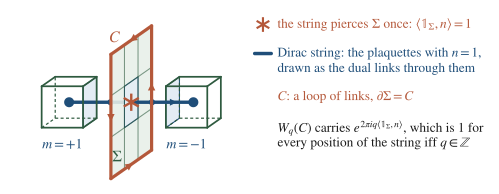
Figure 1. The Villain integer as a Dirac string in $d=3$: it runs from the cube with $m=+1$ to the cube with $m=-1$. A Wilson loop sees it through the phase $e^{2\pi iq⟨1_{\Sigma },n⟩}$, which is 1 for every position of the string exactly when $q$ is an integer.

3. First rewriting: closed electric flux [Computed.]

These are the three moves of Week 3 §2 with $p=2$. Week 2 Problem 8⋆ previewed them; we redo them with every constant because §§4–6 depend on each.

Move 1 — Hubbard–Stratonovich, plaquette by plaquette. With $u_P=(da-2\pi n{)}_P$,

$$e^{-\frac{\beta }{2}{u}_P^2}=\frac{1}{\sqrt{2\pi \beta }}{\int }_{-\infty }^{\infty }d{b}_P{e}^{-\frac{1}{2\beta }{b}_P^2+i{b}_P{u}_P},$$

so that, with $N_P$ the number of plaquettes ($3L^3$ in $d=3$, $6L^4$ in $d=4$),

$$Z=(2\pi \beta {)}^{-N_P/2}\prod _{\ell }{\int }_{-\pi }^{\pi }\frac{d{a}_{\ell }}{2\pi }\prod _P\int d{b}_P\sum _n{e}^{-\frac{1}{2\beta }\Vert b{\Vert }^2+i⟨b,da-2\pi n⟩}.$$

Move 2 — the Dirac comb. The identity ${\sum }_{n_P\in \mathbb{Z}}{e}^{-2\pi i{b}_P{n}_P}={\sum }_{b^{\prime }\in \mathbb{Z}}\delta (b_P-b^{\prime })$ (conventions §3) pins the auxiliary field to integers, $b\in C^2(\Lambda ,\mathbb{Z})$. (Week 3 calls the corresponding integer current $m$, and Week 2 Problem 8⋆ already writes $b$; here $m$ is the monopole number of conventions §4.) Then

$$Z=(2\pi \beta {)}^{-N_P/2}\prod _{\ell }{\int }_{-\pi }^{\pi }\frac{d{a}_{\ell }}{2\pi }\sum _{b\in C^2(\Lambda ,\mathbb{Z})}{e}^{-\frac{1}{2\beta }\Vert b{\Vert }^2+i⟨b,da⟩}.$$

Move 3 — the compact integral gives a Kronecker delta. By adjointness $⟨b,da⟩=⟨\delta b,a⟩={\sum }_{\ell }(\delta b{)}_{\ell }{a}_{\ell }$, where $(\delta b{)}_{\ell }$ is an integer, and ${\int }_{-\pi }^{\pi }\frac{d{a}_{\ell }}{2\pi }{e}^{i(\delta b{)}_{\ell }{a}_{\ell }}={\delta }_{(\delta b{)}_{\ell },0}$. Therefore

$$\boxed{Z=(2\pi \beta {)}^{-N_P/2}\sum _{\begin{array}{c}b\in C^2(\Lambda ,\mathbb{Z})\\ \delta b=0\end{array}}{e}^{-\frac{1}{2\beta }\Vert b{\Vert }^2}.}$$

The integer $b_P$ is the electric flux through $P$ in units of the charge quantum, and $\delta b=0$ at every link says that the flux surfaces are closed. The gauge redundancy needed no fixing: its orbits are compact, and the $a$ integral over them is part of the Kronecker delta. (With $a$ over $\mathbb{R}$ and all $n$ summed, Move 3 would give $\delta ((\delta b{)}_{\ell })$ instead, a Dirac delta evaluated on integers and infinite at $\delta b=0$: the overcounting of §2.1.)

Physical picture. The factor $e^{-b^2/2\beta }$ is the Villain character coefficient of one plaquette, the counterpart of $I_b(\beta )/I_0(\beta )$ for the Wilson action (Week 6), so the boxed sum is the strong-coupling expansion resummed to all orders: a gas of closed integer surfaces of electric flux, weighted by $e^{-(\text{area})/2\beta }$ at unit flux. At small β only small surfaces survive, the confining vacuum of Week 6. In a time slicing, $b$ on a time-like plaquette is the integer electric field $E_{\ell }$ of Week 7 on its spatial link; $\delta b=0$ on the time-like links is Gauss’s law, and on the spatial links it says that $E$ changes only through the magnetic plaquettes. What large β does is decided by the solution of the constraint, which depends on $d$.

4. Three dimensions: heights, monopoles and the dual photon

In $d=3$ the Hodge map sends plaquettes to dual links, and $\delta =+\star d\star$ on 2-cochains (conventions §2, $(-1{)}^{3\cdot 3+1}=+1$). Thus $\delta b=0$ is equivalent to $d(\star b)=0$: $\star b$ is a closed integer 1-cochain on ${\Lambda }^{\ast }$, whose $N^{\ast }=L^3$ sites $\tilde{x}$ are the centers of the cubes of Λ.

4.1 Integer heights and three windings [Proved.]

Claim. Every $b\in C^2(\Lambda ,\mathbb{Z})$ with $\delta b=0$ can be written uniquely as

$$b=\star (d\tilde{h}+\sum _{i=1}^3{w}_i{\tilde{M}}^{(i)}),\tilde{h}\in C^0({\Lambda }^{\ast },\mathbb{Z})\text{modulo a global shift},w\in {\mathbb{Z}}^3,$$

where ${\tilde{M}}^{(i)}$ is a fixed integer 1-cochain on ${\Lambda }^{\ast }$ with unit winding around the $i$-th cycle and none around the others, for instance 1 on the dual links in direction $i$ that cross one chosen plane ${\tilde{x}}_i=\text{const}$, and 0 elsewhere.

Proof. It is Week 3 §3 with $\star b$ in place of $\star m$: measure the three windings $w_i$ of the closed cochain $\star b$, subtract ${\sum }_i{w}_i{\tilde{M}}^{(i)}$, and integrate the closed zero-winding remainder along dual paths from a base site; the result $\tilde{h}$ is path-independent and integer, unique up to its value at the base site. Applying ⋆ once more uses $\star \star =+1$ on these degrees. $\square$

Since ⋆ is a signed bijection of cells, $\Vert \star f\Vert =\Vert f\Vert$, and

$$Z=(2\pi \beta {)}^{-N_P/2}\sum _{w\in {\mathbb{Z}}^3}\sum _{\tilde{h}\in {\mathbb{Z}}^{N^{\ast }}/\mathbb{Z}\cdot 1}\exp (-\frac{1}{2\beta }\Vert d\tilde{h}+w\cdot \tilde{M}{\Vert }^2),$$

the three-dimensional discrete Gaussian model: integer heights at the cube centers, whose level surfaces are the closed flux surfaces of §3. The constraint has no exceptions, so no monopole appears at this stage (Week 2 §7.2, step 4).

4.2 The second Poisson resummation and the zero mode [Computed.]

Move 4 — Poisson on the heights. The heights live on the quotient ${\mathbb{Z}}^{N^{\ast }}/\mathbb{Z}\cdot 1$. As in Week 3 §4 we write the quotient sum as ${\sum }_{\tilde{h}\in {\mathbb{Z}}^{N^{\ast }}}F(\tilde{h})\rho (⟨\tilde{h},1⟩/N^{\ast })$ with ${\sum }_{k\in \mathbb{Z}}\rho (t+k)=1$, Poisson-resum every height, and fold the integral along $1$ back into one period, which is allowed because the integrand is invariant under $\tilde{\phi }\to \tilde{\phi }+1$ for integer $v$. The result is

$$\sum _{\tilde{h}\in {\mathbb{Z}}^{N^{\ast }}/\mathbb{Z}\cdot 1}F(\tilde{h})=\sum _{v\in C^0({\Lambda }^{\ast },\mathbb{Z})}{\int }_{{\mathbb{R}}^{N^{\ast }}/\mathbb{Z}\cdot 1}{d}^{N^{\ast }}\tilde{\phi }F(\tilde{\phi })e^{2\pi i⟨v,\tilde{\phi }⟩},F(\tilde{\phi })=e^{-\frac{1}{2\beta }\Vert d\tilde{\phi }+w\cdot \tilde{M}{\Vert }^2},$$

with one integer $v_{\tilde{x}}$ per dual site, that is, one per cube of Λ.

Move 5 — the zero mode runs over one period. Write $\tilde{\phi }={\tilde{\phi }}_{0}1+{\tilde{\phi }}^{\prime }$ with ${\tilde{\phi }}^{\prime }\perp 1$ and ${\tilde{\phi }}_0\in [0,1)$. The coordinate along the unit vector $1/\sqrt{N^{\ast }}$ is $\sqrt{N^{\ast }}{\tilde{\phi }}_0$, so $d^{N^{\ast }}\tilde{\phi }=\sqrt{N^{\ast }}d{\tilde{\phi }}_0{d}^{N^{\ast }-1}{\tilde{\phi }}^{\prime }$. $F$ does not depend on ${\tilde{\phi }}_0$, and

$$\sqrt{N^{\ast }}{\int }_0^{1}d{\tilde{\phi }}_0{e}^{2\pi i{\tilde{\phi }}_0{\sum }_{\tilde{x}}{v}_{\tilde{x}}}=\sqrt{N^{\ast }}{\delta }_{{\sum }_{\tilde{x}}{v}_{\tilde{x}},0},$$

a Kronecker delta, because $\sum v$ is an integer. The integers are neutral configuration by configuration, and in each winding sector

$$Z^{(w)}=(2\pi \beta {)}^{-N_P/2}\sqrt{N^{\ast }}\sum _{\begin{array}{c}v\in C^0({\Lambda }^{\ast },\mathbb{Z})\\ \sum v=0\end{array}}{\int }_{{\tilde{\phi }}^{\prime }\perp 1}{d}^{N^{\ast }-1}{\tilde{\phi }}^{\prime }{e}^{-\frac{1}{2\beta }\Vert d{\tilde{\phi }}^{\prime }+w\cdot \tilde{M}{\Vert }^2+2\pi i⟨v,{\tilde{\phi }}^{\prime }⟩}.$$

Integrating ${\tilde{\phi }}_0$ over $\mathbb{R}$, as if the heights were not defined modulo a shift, would give $\delta (\sum v)$, a Dirac delta evaluated on an integer (Week 3 F4).

4.3 The Poisson integers are the monopoles [Proved.]

The integers $v$ and the Villain integers $n$ are different summation variables. What can be proved exactly is that $v$ carries the weights of the monopole numbers $m=dn$. Add a source $e^{i⟨\eta ,dn⟩}$ to the Villain weight, with $\eta \in C^3(\Lambda ,\mathbb{R})$ arbitrary. Since $⟨\eta ,dn⟩=⟨\delta \eta ,n⟩$, Move 2 becomes ${\sum }_n{e}^{-2\pi i⟨b-\delta \eta /2\pi ,n⟩}$, which pins $b=b^{\prime }+\delta \eta /2\pi$ with $b^{\prime }$ integer, and Move 3 gives $\delta b^{\prime }=0$ because ${\delta }^2=0$. In $d=3$, $\delta =-\star d\star$ on 3-cochains (conventions §2), so with $\tilde{\eta }=\star \eta \in C^0({\Lambda }^{\ast },\mathbb{R})$ the weight is

$$\exp (-\frac{1}{2\beta }\Vert \star b^{\prime }+\star \delta \eta /2\pi {\Vert }^2)=\exp (-\frac{1}{2\beta }\Vert d(\tilde{h}-\tilde{\eta }/2\pi )+w\cdot \tilde{M}{\Vert }^2).$$

After Move 4 the shift $\tilde{\phi }\to \tilde{\phi }+\tilde{\eta }/2\pi$ removes $\tilde{\eta }$ from $F$ and moves it into the source, $e^{2\pi i⟨v,\tilde{\phi }⟩}\to e^{i⟨v,\tilde{\eta }⟩}{e}^{2\pi i⟨v,\tilde{\phi }⟩}$. Both sides of the resulting identity are Fourier series in $\eta \in (\mathbb{R}/2\pi \mathbb{Z}{)}^{N_C}$, with $N_C$ the number of cubes. On the Villain side the coefficient of $e^{i⟨\eta ,m⟩}$ is the total weight of the configurations with $dn=m$; on the dual side, since $⟨v,\star \eta ⟩=⟨{\star }^{-1}v,\eta ⟩$, it is the total dual weight of $v=\star m$. Equal Fourier series have equal coefficients, so

$$\boxed{{\text{weight}}_{\mathrm{Villain}}(dn=m)={\text{weight}}_{\mathrm{dual}}(v=\star m)\text{for every }m\in C^3(\Lambda ,\mathbb{Z}),v_{c^{\ast }}=m_c,}$$

with sign $+1$, since $ϵ(\{1,2,3\},\varnothing )=+1$. The monopole of the cube $c$ sits at the dual site $c^{\ast }$ at its center (Figure 2), and the neutrality of Move 5 is the identity ${\sum }_c{m}_c=0$ of §2.1.

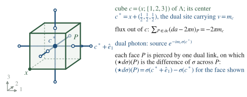
Figure 2. Where a three-dimensional monopole lives: the integer $m_c=(dn{)}_c$ of a cube becomes the Poisson integer $v$ at the dual site at its center, and couples to the dual photon as $e^{-i{m}_c\sigma (c^{\ast })}$.

4.4 The monopole Coulomb gas [Computed.]

Move 6 — integrate the smooth dual field. In the $w=0$ sector the ${\tilde{\phi }}^{\prime }$ integral is Gaussian with source $2\pi v$. With Δ the Laplacian of ${\Lambda }^{\ast }$ ($\Delta \ge 0$) and $G^{\prime }$ its inverse on the complement of the constants, the shift ${\tilde{\phi }}^{\prime }={\tilde{\phi }}^{\prime \prime }+2\pi i\beta G^{\prime }v$ completes the square exactly as in Week 3 Move 6, and

$$\boxed{Z^{(0)}=(2\pi \beta {)}^{-N_P/2}{Z}_{\mathrm{ph}}\sum _{\begin{array}{c}v\in C^0({\Lambda }^{\ast },\mathbb{Z})\\ \sum v=0\end{array}}{e}^{-2{\pi }^2\beta ⟨v,G^{\prime }v⟩},Z_{\mathrm{ph}}=\sqrt{N^{\ast }}(2\pi \beta {)}^{(N^{\ast }-1)/2}(\det {}^{\prime }\Delta {)}^{-1/2},}$$

where $Z_{\mathrm{ph}}$ is the free dual-photon partition function, Jacobian of Move 5 included, and $\det {}^{\prime }\Delta$ is the product of the nonzero eigenvalues of Δ. (On the $2^3$ torus at $\beta =0.6$ the height sum of §4.1 and this Coulomb-gas form both equal $1.1629774772$ once the common factor $(2\pi \beta {)}^{-N_P/2}$ is removed, a check of $\sqrt{N^{\ast }}$ and of the determinant.)

Move 7 — the monopole action and the Coulomb law. Unlike $d=2$, the three-dimensional Green function is finite at the origin, so no subtraction is needed:

$$2{\pi }^2\beta ⟨v,G^{\prime }v⟩=2{\pi }^2\beta G^{\prime }(0)\sum _{\tilde{x}}{v}_{\tilde{x}}^2+4{\pi }^2\beta \sum _{\{\tilde{x},\tilde{y}\}}{v}_{\tilde{x}}{v}_{\tilde{y}}{G}^{\prime }(\tilde{x}-\tilde{y}),$$

where the last sum runs over unordered pairs of distinct dual sites. On the infinite lattice $G^{\prime }\to G_3$, with $G_3(0)=0.252731$ and $G_3(r)\to 1/4\pi r$ (conventions §2), so each unit monopole costs

$$\boxed{S_{\mathrm{mono}}=2{\pi }^2{G}_3(0)\beta =4.99\beta }$$

and two monopoles interact through $4{\pi }^2\beta q_i{q}_j{G}_3(r_{ij})$, where $q_i{q}_j=m_i{m}_j$. In physical units $\beta =1/e^2{a}_{\mathrm{lat}}$ and $G_3$ at lattice separation $r/a_{\mathrm{lat}}$ tends to $a_{\mathrm{lat}}/4\pi r$, so the pair energy is $\frac{4{\pi }^2}{e^2}{q}_i{q}_j\frac{1}{4\pi r}$, the Coulomb law of magnetic charges $2\pi /e$ of conventions §5. There is no fluctuation determinant around a monopole: the Villain photon and the monopoles decouple exactly, so $e^{-S_{\mathrm{mono}}}$ is the complete weight of a unit monopole on its dual site. The fugacity per unit volume of Week 9 is $\zeta =e^{-S_{\mathrm{mono}}}/a_{\mathrm{lat}}^3$, in the scheme in which vertex operators are normal-ordered at the lattice scale (Week 3 §6).

The same gas from the Villain integers [Proved.]. The Hodge argument of Week 3 §5 gives the Coulomb gas directly from $m=dn$. Decompose $2\pi n=d\alpha +\delta \xi +h$ into exact, coexact and harmonic parts (Week 2 §6), with $\xi \in C^3(\Lambda ,\mathbb{R})$. Orthogonality gives $\Vert da-2\pi n{\Vert }^2=\Vert d(a-\alpha ){\Vert }^2+\Vert \delta \xi {\Vert }^2+\Vert h{\Vert }^2$, and applying $d$ gives $d\delta \xi =2\pi m$. In $d=3$ the cubes are top cells, so $\Delta =d\delta$ on 3-cochains, $\xi =2\pi G^{\prime }m$ (solvable because ${\sum }_c{m}_c=0$), and

$$\Vert \delta \xi {\Vert }^2=⟨\xi ,d\delta \xi ⟩=4{\pi }^2⟨m,G^{\prime }m⟩,\text{so}\underset{a}{\min }\frac{\beta }{2}\Vert da-2\pi n{\Vert }^2=2{\pi }^2\beta ⟨m,G^{\prime }m⟩+\frac{\beta }{2}\Vert h{\Vert }^2,$$

where $G^{\prime }$ is the Green function of Move 6, since ⋆ intertwines the Laplacians, and $h$ is a torus flux term (F4). [Computed.] On the $6^3$ torus (coordinates 0 to 5) take $n=1$ on the three $(2,3)$-plaquettes based at $(2,2,2)$, $(3,2,2)$ and $(4,2,2)$, and $n=0$ elsewhere: the string of Figure 1, with $m=+1$ on the cube based at $(1,2,2)$ and $m=-1$ on the cube based at $(4,2,2)$. Least squares in $a$ gives $\min \Vert da-2\pi n{\Vert }^2=18.60208$, while $4{\pi }^2⟨m,G^{\prime }m⟩=16.95714$ and $\Vert h{\Vert }^2=4{\pi }^2{\Phi }^2/L={\pi }^2/6=1.64493$, with $\Phi =\frac{1}{2}$ the average flux through the $(2,3)$ slices; the flux of the minimizing $F$ out of the two cubes is $-2\pi$ and $+2\pi$.

4.5 The dual photon [Computed.]

Define the dual photon by

$$\sigma =-2\pi \tilde{\phi }\in {\mathbb{R}}^{N^{\ast }}/2\pi \mathbb{Z}\cdot 1,$$

where the sign is chosen to match conventions §5. Moves 4 and 5 then read

$$\boxed{Z=\frac{(2\pi \beta {)}^{-N_P/2}}{(2\pi {)}^{N^{\ast }}}\sum _{w\in {\mathbb{Z}}^3}\sum _{v\in C^0({\Lambda }^{\ast },\mathbb{Z})}{\int }_{{\mathbb{R}}^{N^{\ast }}/2\pi \mathbb{Z}}{d}^{N^{\ast }}\sigma \exp (-\frac{1}{8{\pi }^2\beta }\Vert d\sigma -2\pi w\cdot \tilde{M}{\Vert }^2-i⟨v,\sigma ⟩),v=\star dn,}$$

the dual photon with the monopoles as explicit integers on dual sites, entering as $e^{-i{m}_c\sigma (c^{\ast })}$. Four normalizations follow.

• Stiffness. On smooth configurations ${\sum }_{\tilde{\ell }}(d\sigma {)}_{\tilde{\ell }}^2\to a_{\mathrm{lat}}^{-1}\int d^{3}x(\partial \sigma {)}^2$ and $\frac{1}{8{\pi }^2\beta }=\frac{e^2{a}_{\mathrm{lat}}}{8{\pi }^2}$, so the action is $\frac{e^2}{8{\pi }^2}\int d^{3}x(\partial \sigma {)}^2$, with σ dimensionless and $e^2$ of mass dimension one.
• Periodicity. $\sigma \sim \sigma +2\pi$ because the heights are integers defined modulo a global shift, and equivalently because every monopole charge is an integer, so that $e^{-iv\sigma }$ is $2\pi$-periodic. The periodicity of the dual photon is the magnetic half of the Dirac quantization of §2.2.
• Field strength. From Move 1, $\int dbb{e}^{-b^2/2\beta +ibu}=i\beta u\int db{e}^{-b^2/2\beta +ibu}$, so inserting $b_P$ in the dual representation is inserting $i\beta F_P$ in the original. Carried through Moves 2–5 at $w=0$, $b=\star d\tilde{h}\to \star d\tilde{\phi }=-\star d\sigma /2\pi$, and

$$F=da-2\pi n\simeq \frac{i}{2\pi \beta }\star d\sigma ,$$

where $(\star d\sigma )(P_{\mu \nu })=a_{\mathrm{lat}}{ϵ}_{\mu \nu \rho }{\partial }_{\rho }\sigma$ is the difference of σ across the plaquette along its normal. With $F_{\mu \nu }=a_{\mathrm{lat}}^{-2}F(P_{\mu \nu })$ this is $B_{\mu }=\frac{1}{2}{ϵ}_{\mu \nu \rho }{F}_{\nu \rho }=+\frac{i{e}^2}{2\pi }{\partial }_{\mu }\sigma$, the relation of conventions §5. As a check, the saddle of the σ integral with the source $-i⟨v,\sigma ⟩$ solves $\Delta \sigma =-4{\pi }^{2}i\beta v$, and the flux of $\frac{i}{2\pi \beta }\star d\sigma$ out of a cube is $-\frac{i}{2\pi \beta }(\Delta \sigma )(c^{\ast })=-2\pi m_c$, as §2.1 requires; on the $6^3$ configuration of §4.4 this saddle reproduces the coexact part of the minimizing $F$ exactly.

• Symmetry. The σ action is invariant under $\sigma \to \sigma +c$. This is the magnetic $U(1{)}^{(0)}$ of the form-degree table (conventions §6, higher-form-symmetries): a 0-form symmetry in $d=3$, with current $F/2\pi =\frac{i}{4{\pi }^2\beta }\star d\sigma$ and local charged operators $e^{iq\sigma (\tilde{x})}$, the monopole operators. The monopole sources $e^{-i{m}_c\sigma }$ carry charge $-m_c$ and break it explicitly; without them σ would be the Goldstone boson of its spontaneous breaking.

Physical picture. The height model of §4.1 carries Week 3’s rough and smooth surfaces into three dimensions with one change. A Wilson loop inserts a surface across which the heights jump (Problem 1), so an area law for $W(C)$ is a finite interface tension of the height model, and a gapped dual photon is a pinned height field. In $d=2$ the heights roughen at large β, and that is the BKT transition of Week 4. In $d=3$ the integer structure, carried by the sources $e^{-im\sigma }$, pins σ at every β, with a correlation length that grows like $e^{S_{\mathrm{mono}}/2}$ at weak coupling: Polyakov’s mechanism in the height variables. The dictionary is exact; confinement at every coupling is the theorem of Göpfert and Mack [Stated — refs.], and the controlled weak-coupling calculation is Week 10.

5. Four dimensions: the Banks–Myerson–Kogut duality

In $d=4$ the Hodge map sends plaquettes to dual plaquettes (degree 2 is self-dual, Week 2 §5.1), and $\delta =-\star d\star$ on 2-cochains (conventions §2), so $\delta b=0$ is again $d(\star b)=0$, now for an integer 2-cochain on ${\Lambda }^{\ast }$.

5.1 The integer 2-form and its $\mathbb{Z}$ gauge field [Proved.]

Claim. Every $b\in C^2(\Lambda ,\mathbb{Z})$ with $\delta b=0$ can be written as

$$b=\star (d\tilde{N}+\sum _{i<j}{w}_{ij}{\tilde{M}}^{(ij)}),\tilde{N}\in C^1({\Lambda }^{\ast },\mathbb{Z}),w\in {\mathbb{Z}}^6,$$

with $w$ unique and $\tilde{N}$ unique modulo the closed integer 1-cochains $Z^1({\Lambda }^{\ast },\mathbb{Z})$ (the integer gauge transformations $\tilde{N}\to \tilde{N}+d\tilde{k}$ and the four integer windings), where ${\tilde{M}}^{(ij)}$ is 1 on the $(ij)$ dual plaquettes at one fixed position in the $(ij)$ plane, for all values of the other two coordinates, and 0 elsewhere.

Proof. ${\tilde{M}}^{(ij)}$ is closed, since it does not vary along the other two directions, and its period is 1 on the 2-tori spanned by $(i,j)$ and 0 on the other five kinds. Subtracting $\sum w_{ij}{\tilde{M}}^{(ij)}$, with $w_{ij}$ the periods of $\star b$, leaves a closed integer cochain with zero periods. Since $H^2(T^4,\mathbb{Z})={\mathbb{Z}}^6$ has no torsion (Week 2 §4.3), that cochain is $d\tilde{N}$ with $\tilde{N}$ integer, unique up to closed integer 1-cochains; and $\star \star =+1$ on 2-cochains in $d=4$. $\square$

Therefore

$$Z=(2\pi \beta {)}^{-N_P/2}\sum _{w\in {\mathbb{Z}}^6}\sum _{\tilde{N}\in C^1({\Lambda }^{\ast },\mathbb{Z})/Z^1({\Lambda }^{\ast },\mathbb{Z})}\exp (-\frac{1}{2\beta }\Vert d\tilde{N}+w\cdot \tilde{M}{\Vert }^2),$$

a $\mathbb{Z}$ gauge theory on the dual lattice with Gaussian action, the four-dimensional counterpart of the heights.

5.2 The second resummation and the gauge quotient [Computed.]

The sum runs over the lattice $C^1({\Lambda }^{\ast },\mathbb{Z})$ modulo its sublattice $\Gamma =Z^1({\Lambda }^{\ast },\mathbb{Z})$, which spans the space $W=Z^1({\Lambda }^{\ast },\mathbb{R})$ of closed real 1-cochains, and the summand is invariant under translations by $W$. Moves 4 and 5 generalize directly. Choose ρ on $W$ with ${\sum }_{\gamma \in \Gamma }\rho (\omega +\gamma )=1$, write the quotient sum as ${\sum }_{\tilde{N}}F(\tilde{N})\rho (P_W\tilde{N})$ with $P_W$ the orthogonal projector onto $W$, and Poisson-resum every dual link:

$$\sum _{\tilde{N}\in C^1(\mathbb{Z})/\Gamma }F(\tilde{N})=\sum _{j\in C^1({\Lambda }^{\ast },\mathbb{Z})}{\int }_{C^1(\mathbb{R})/\Gamma }d\tilde{A}F(\tilde{A})e^{2\pi i⟨j,\tilde{A}⟩}.$$

Split $\tilde{A}=\omega +{\tilde{A}}_{\perp }$ with $\omega \in W$ (pure gauge and flat) and ${\tilde{A}}_{\perp }\perp W$ (coexact). $F$ depends only on $d\tilde{A}=d{\tilde{A}}_{\perp }$, and for integer $j$ the function $e^{2\pi i⟨j,\omega ⟩}$ is Γ-periodic on $W$, so

$${\int }_{W/\Gamma }d\omega e^{2\pi i⟨j,\omega ⟩}=c_4{\delta }_{P_{W}j,0},c_4=\mathrm{vol}(W/\Gamma ).$$

Since $⟨j,d\tilde{\lambda }⟩=⟨\delta j,\tilde{\lambda }⟩$, the condition $P_{W}j=0$ says that $j$ is conserved, $\delta j=0$ at every dual site, and has zero net winding around each of the four cycles. Therefore

$$Z^{(w)}=(2\pi \beta {)}^{-N_P/2}{c}_4\sum _{\begin{array}{c}j\in C^1({\Lambda }^{\ast },\mathbb{Z})\\ \delta j=0,\text{no winding}\end{array}}{\int }_{\mathrm{coexact}}d{\tilde{A}}_{\perp }{e}^{-\frac{1}{2\beta }\Vert d{\tilde{A}}_{\perp }+w\cdot \tilde{M}{\Vert }^2+2\pi i⟨j,{\tilde{A}}_{\perp }⟩},$$

where the β-independent constant $c_4$ plays the part of $\sqrt{N^{\ast }}$ (F2).

5.3 The monopole current [Proved.]

The source argument of §4.3 runs unchanged. With $e^{i⟨\eta ,dn⟩}$, $\eta \in C^3(\Lambda ,\mathbb{R})$, Move 2 pins $b=b^{\prime }+\delta \eta /2\pi$; in $d=4$, $\delta =-\star d\star$ on 3-cochains, so $\star b=d(\tilde{N}-\star \eta /2\pi )+w\cdot \tilde{M}$ with $\star \eta \in C^1({\Lambda }^{\ast },\mathbb{R})$, and the shift $\tilde{A}\to \tilde{A}+\star \eta /2\pi$ moves it into the source as $e^{i⟨j,\star \eta ⟩}$. Comparing Fourier coefficients in η,

$$\boxed{j=\star m=\star dn:\text{the conserved integer current on dual links is the monopole current.}}$$

Its conservation is the Bianchi identity, $\delta j=-\star d\star \star dn=\star d(dn)=0$ (with $\star \star =-1$ on 3-cochains in $d=4$), and its zero winding says that monopole loops bound Dirac sheets.

Where it sits (Figure 3). The dual of the cube $(x;S)$, $|S|=3$, is the dual link based at $x+\frac{1}{2}{\hat{e}}_S-\frac{1}{2}{\hat{e}}_{S^c}$ in the single direction $S^c$, with sign $ϵ(S,S^c)$. For the spatial cube $(x;\{1,2,3\})$ it runs from $x+\frac{1}{2}(1,1,1,-1)$ to $x+\frac{1}{2}(1,1,1,1)$, straight through the cube in the $+4$ direction: a monopole sitting in that cube at time $x_4$ is one step of a worldline in time. The four orientations give

$$j_4=+m_{123},j_3=-m_{124},j_2=+m_{134},j_1=-m_{234},$$

where $m_{\mu \nu \rho }$ is $m$ on the cube spanned by $\mu <\nu <\rho$ (checked cell by cell on the $3^4$ torus).

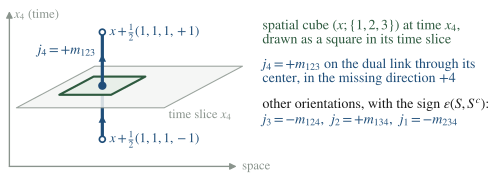
Figure 3. Where a four-dimensional monopole lives: the cube $(x;S)$ is dual to the dual link through its center in the missing direction, and $m$ on the cube becomes the monopole current $j=\star m$ on that link, with the shuffle sign $ϵ(S,S^c)$.

5.4 The dual gauge field at $\tilde{\beta }=1/4{\pi }^2\beta$ [Computed.]

Define $\tilde{a}=-2\pi \tilde{A}$, with the same sign convention as σ. Then

$$\frac{1}{2\beta }\Vert d\tilde{A}+w\cdot \tilde{M}{\Vert }^2=\frac{\tilde{\beta }}{2}\Vert d\tilde{a}-2\pi w\cdot \tilde{M}{\Vert }^2,\boxed{\tilde{\beta }=\frac{1}{4{\pi }^2\beta },\tilde{e}=\frac{2\pi }{e},}$$

and the source is $e^{2\pi i⟨j,\tilde{A}⟩}=e^{-i⟨j,\tilde{a}⟩}$: the monopole current couples to the dual gauge field as the current of a Wilson loop. In $d=4$, $\beta =1/e^2$ is dimensionless and $\tilde{\beta }=e^2/4{\pi }^2=1/{\tilde{e}}^2$, so $e\tilde{e}=2\pi$, the Dirac condition for the minimal electric and magnetic charges; the map is an involution, $\widetilde{\stackrel{~}{\beta }}=\beta$. The insertion argument of §4.5 gives the lattice duality relation

$$F=da-2\pi n\simeq \frac{i}{2\pi \beta }\star d\tilde{a}=2\pi i\tilde{\beta }\star d\tilde{a},$$

which in the continuum is $F=\frac{i{e}^2}{2\pi }\star \tilde{F}$: each field strength is the Hodge dual of the other, up to the $i$ of Euclidean signature (checked at the saddle on the $4^4$ configuration of §5.5). The winding sectors enter as the closed integer 2-cochain $\tilde{n}=w\cdot \tilde{M}$ in the Villain combination $d\tilde{a}-2\pi \tilde{n}$, so they are the magnetic flux sectors of the dual photon, and the dual theory has no monopoles of its own, $d\tilde{n}=0$ (§6 makes this exact). Gauge invariance of $e^{-i⟨j,\tilde{a}⟩}$ under $\tilde{a}\to \tilde{a}+d\tilde{\lambda }$ is the conservation $\delta j=0$, the Bianchi identity of the original, and its invariance under $\tilde{a}\to \tilde{a}+2\pi \tilde{k}$ is the integrality of $j$, the original’s Dirac quantization.

5.5 The monopole loop gas [Computed.]

On a hypercubic lattice the Laplacian of 1-cochains acts on each component as the site Laplacian. With ${\nabla }_{\mu }f(x)=f(x+\hat{\mu })-f(x)$ and ${\nabla }_{\mu }^{\ast }f(x)=f(x)-f(x-\hat{\mu })$ we have $(\delta dA{)}_{\nu }=-{\sum }_{\mu }{\nabla }_{\mu }^{\ast }({\nabla }_{\mu }{A}_{\nu }-{\nabla }_{\nu }{A}_{\mu })$ and $(d\delta A{)}_{\nu }=-{\nabla }_{\nu }{\sum }_{\mu }{\nabla }_{\mu }^{\ast }{A}_{\mu }$, whose sum is $(\Delta A{)}_{\nu }=-{\sum }_{\mu }{\nabla }_{\mu }^{\ast }{\nabla }_{\mu }{A}_{\nu }$. On coexact cochains $\Vert d{\tilde{A}}_{\perp }{\Vert }^2=⟨{\tilde{A}}_{\perp },\Delta {\tilde{A}}_{\perp }⟩$, so the Gaussian integral of §5.2 at $w=0$ with source $2\pi j$ gives, exactly as in Move 6,

$$\boxed{Z^{(0)}=(2\pi \beta {)}^{-N_P/2}{c}_4(2\pi \beta {)}^{r/2}\left(\det {\Delta }_{\mathrm{coex}}{)}^{-1/2}\sum _{\begin{array}{c}j\in C^1({\Lambda }^{\ast },\mathbb{Z})\\ \delta j=0,\text{no winding}\end{array}}\exp \right(-2{\pi }^2\beta \sum _{\mu =1}^4⟨j_{\mu },G^{\prime }{j}_{\mu }⟩),}$$

where $r$ is the dimension of the space of coexact 1-cochains on ${\Lambda }^{\ast }$ and ${\Delta }_{\mathrm{coex}}$ is Δ restricted to it. This is the BMK representation: free photons times a gas of closed monopole loops. Two current elements interact only when parallel, through $4{\pi }^2\beta G_4(r)\to \beta /r^2$ at large separation (the four-dimensional Coulomb law), and each link of a loop carries the self-energy

$$2{\pi }^2{G}_4(0)\beta =3.06\beta ,$$

with $G_4(0)=0.154933$, the number that enters the energy–entropy estimate of Week 11 and Problem 4⋆. The Hodge argument of §4.4 carries over, with $\xi$ chosen exact so that $\Delta \xi =d\delta \xi$. [Computed.] On the $4^4$ torus take $n=1$ on the $(3,4)$-plaquettes based at $(0,0,1,1)$ and $(1,0,1,1)$: $j=\star dn$ is a rectangular loop of six dual links in a $(1,2)$ plane, and least squares in $a$ gives $\min \Vert da-2\pi n{\Vert }^2=34.19113=33.57428+{\pi }^2/16$, where $33.57428=4{\pi }^2{\sum }_{\mu }⟨j_{\mu },G^{\prime }{j}_{\mu }⟩$ and ${\pi }^2/16=4{\pi }^2{\Phi }^2$ is the flux term, with average flux $\Phi =\frac{1}{8}$.

Physical picture. Read as a theory of the dual photon $\tilde{a}$, the loops $j$ are its charged particles, and the phases of Week 11 are phases of a gauge theory with matter. At weak coupling a link costs $3.06\beta$, the loops are small and rare, and $\tilde{a}$, and with it the photon, stays massless: the Coulomb phase. At strong coupling long loops are cheap and entropically favoured; a condensate of the dual charges Higgses $\tilde{a}$, and through $F\simeq 2\pi i\tilde{\beta }\star d\tilde{a}$ the original electric flux is squeezed into tubes, the dual-superconductor. The representation is exact; the transition and its location are Week 11’s energy–entropy argument and Guth’s theorem [Stated — refs.].

6. Electric–magnetic duality at the Villain level [Proved.]

The self-duality of degree 2 in $d=4$ now becomes an identity with every constant. Define the monopole-free Villain gauge theory on ${\Lambda }^{\ast }$ with a background current $j$,

$${\tilde{Z}}_{\tilde{\beta }}[j]=\prod _{\tilde{\ell }}{\int }_{-\pi }^{\pi }\frac{d{\tilde{a}}_{\tilde{\ell }}}{2\pi }\sum _{\begin{array}{c}\tilde{n}\in C^2({\Lambda }^{\ast },\mathbb{Z})\\ d\tilde{n}=0\end{array}}\exp (-\frac{\tilde{\beta }}{2}\Vert d\tilde{a}-2\pi \tilde{n}{\Vert }^2-i⟨j,\tilde{a}⟩),$$

where the constraint $d\tilde{n}=0$ removes its monopoles. Then

$$\boxed{Z_{\beta }=(2\pi \beta {)}^{-N_P/2}\sum _{j\in C^1({\Lambda }^{\ast },\mathbb{Z})}{\tilde{Z}}_{\tilde{\beta }}[j],\tilde{\beta }=\frac{1}{4{\pi }^2\beta }.}$$

Proof. On each dual link ${\sum }_{j\in \mathbb{Z}}{e}^{-ij\tilde{a}}=2\pi {\sum }_{k\in \mathbb{Z}}\delta (\tilde{a}-2\pi k)$, which on $(-\pi ,\pi ]$ sets $\tilde{a}=0$ with unit weight against $d\tilde{a}/2\pi$. The right side is therefore $(2\pi \beta {)}^{-N_P/2}{\sum }_{d\tilde{n}=0}{e}^{-2{\pi }^2\tilde{\beta }\Vert \tilde{n}{\Vert }^2}$, and $2{\pi }^2\tilde{\beta }=1/2\beta$. By §3 and §5.1 the left side is the same sum, over all closed integer 2-cochains $\star b$ of ${\Lambda }^{\ast }$. $\square$

The proof sums over $j$ first. Integrating $\tilde{a}$ first at fixed $j$ instead, the redundancy $\tilde{a}\to \tilde{a}+2\pi \tilde{k}$, $\tilde{n}\to \tilde{n}+d\tilde{k}$ unfolds the exact part of $\tilde{n}$ into $\tilde{a}\in \mathbb{R}$, the compact gauge and flat directions give $c_4{\delta }_{P_{W}j,0}$ as in §5.2, and what remains is the Gaussian of §5.5, term by term; §5.3 identified $j$ with $\star dn$. The identity is thus the explicit statement of electric–magnetic duality for the Villain theory: Villain $U(1)$ at β, with dynamical monopoles and no electric charges, is Villain $U(1)$ on ${\Lambda }^{\ast }$ at $\tilde{\beta }=1/4{\pi }^2\beta$, with dynamical electric worldlines (the original monopoles, summed with unit weight and no action of their own) and no monopoles. Weak coupling maps to strong coupling. Its limitation is the asymmetry of the matter. The monopoles of the dual theory would be the electric charges of the original, which pure gauge theory lacks; the pure theory is therefore not self-dual, and the coupling $\beta =1/2\pi$ fixed by the map is not a symmetric point of it. A model with both kinds of matter is self-dual (Problem 6⋆⋆).

The three-dimensional identity has the same proof, with σ in place of $\tilde{a}$:

$$Z_{\beta }=(2\pi \beta {)}^{-N_P/2}\sum _{v\in C^0({\Lambda }^{\ast },\mathbb{Z})}{\tilde{Z}}_{\tilde{\beta }}^{\mathrm{XY}}[v],{\tilde{Z}}_{\tilde{\beta }}^{\mathrm{XY}}[v]=\prod _{\tilde{x}}{\int }_{-\pi }^{\pi }\frac{d{\sigma }_{\tilde{x}}}{2\pi }\sum _{\begin{array}{c}\tilde{n}\in C^1({\Lambda }^{\ast },\mathbb{Z})\\ d\tilde{n}=0\end{array}}{e}^{-\frac{\tilde{\beta }}{2}\Vert d\sigma -2\pi \tilde{n}{\Vert }^2-i⟨v,\sigma ⟩},$$

and unfolding it at fixed $v$ returns the boxed form of §4.5. Compact QED₃ is the vortex-free Villain XY model of its dual photon, with the monopoles as its charges; the vortices of σ would be the electric charges, and a Wilson loop is a vortex line of σ (Problem 1). In $d=4$ the Wilson loop of $a$ is likewise a monopole worldline of $\tilde{a}$, its ‘t Hooft loop. The operator content, checked against the form-degree table of conventions §6 (magnetic symmetry of degree $d-3$ for a $U(1)$ gauge field, winding symmetry of degree $d-2$ for a compact scalar), extends the dictionary of Week 3 §8:

model	dual variables	defect and its location	magnetic (winding) symmetry	fate
2d XY (Week 3)	heights, χ on dual sites	vortex $v=dn\in C^2$, at dual sites	0-form; local vortex operators $e^{i\chi }$	BKT (Week 4)
3d $U(1)$	heights, σ on dual sites	monopole $m=dn\in C^3$, at dual sites	0-form; local monopole operators $e^{i\sigma }$	confining at every β (Weeks 9–10)
4d $U(1)$	$\mathbb{Z}$ gauge field, $\tilde{a}$ on dual links	monopole current $j=\star dn$, closed dual loops	1-form; ‘t Hooft lines	Coulomb and confining phases (Week 11)

Each row is an exact identity of partition functions. In each dual description the monopoles are charged matter, and they break the magnetic symmetry explicitly; the electric 1-form symmetry of $a$ is, in $d=3$, the winding symmetry of σ (degree $d-2=1$, charged objects the Wilson lines) and, in $d=4$, the magnetic 1-form symmetry of $\tilde{a}$. Semester II Week 12 removes the defects altogether (modified Villain) and makes the symmetries exact on the lattice. Figure 4 assembles the chain.

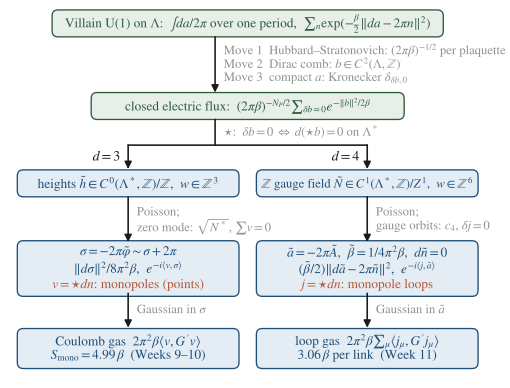
Figure 4. The duality chain of this week: one set of moves, two constraint solutions, and the defects of the original theory returning as the integers of the second resummation.

7. Subtleties and fine print

F1 — Where the monopole sits, and its sign. In $d=3$, $v_{c^{\ast }}=+m_c$ at the center of the cube; the lattice number $m_c$ is minus the magnetic charge, so the monopole operator $e^{i\sigma (\tilde{x})}$ inserts $q=+1$, a unit of $m=-1$ forced at that cube, which on the direct side is a disorder operator (a Dirac string ending at the cube, whose position is a redundancy). In $d=4$ the current sits on the dual link through the cube in the missing direction, with the shuffle sign of §5.3. The signs matter as soon as monopole currents are coupled to anything else, for instance the θ-term and the Witten effect of Week 12, where a wrong sign flips the induced electric charge.

F2 — Gauge fixing the dual description. The Poisson-dual fields inherit the redundancies of the integers they replace: the global shift of the heights in $d=3$, and the integer gauge transformations and windings of $\tilde{N}$ in $d=4$. Summing over the quotient, as the claims of §§4.1 and 5.1 require, makes the corresponding directions of the real field compact: a circle of length $\sqrt{N^{\ast }}$ for the zero mode of $\tilde{\phi }$, and the torus $W/\Gamma$ of volume $c_4$ for the gauge and flat directions of $\tilde{A}$. Integrating over them gives Kronecker constraints (neutrality; $\delta j=0$ with zero winding) and the constants; what remains is $\tilde{A}$ in the Landau gauge $\delta \tilde{A}=0$ without harmonic part, and no Faddeev–Popov determinant appears. The constant is $c_4=\sqrt{\tau }{L}^4$, with τ the number of spanning trees of ${\Lambda }^{\ast }$ ($\tau =\det {}^{\prime }{\Delta }_0/N^{\ast }$ by the matrix-tree theorem): the exact integer 1-cochains have covolume $\sqrt{\tau }$, and each of the four unit windings projects on the harmonic space with norm $L$. (The same identity for 1-cochains on the $2\times 2$ torus in $d=2$, where the constant is $\sqrt{32}$, holds to ten digits.) Treating $\tilde{A}$ as an unconstrained real field would multiply $Z$ by the infinite volume of the gauge orbits, the dual-side form of the non-compact-measure error named in the instructor checkpoint.

F3 — The fate of the Maxwell normalization. In $d=3$ the dual stiffness is $\tilde{\beta }=1/4{\pi }^2\beta$ per dual link, $\frac{e^2}{8{\pi }^2}$ in the continuum, of mass dimension one. In $d=4$ the Maxwell coefficient $\frac{1}{2e^2}$ becomes $\frac{1}{2{\tilde{e}}^2}=\frac{e^2}{8{\pi }^2}$; the naive guess $e\to 1/e$ misses the factor $2\pi$, which is Dirac’s. Since $(2\pi \beta {)}^{-N_P/2}=(2\pi \tilde{\beta }{)}^{N_P/2}$, the identity of §6 can be written symmetrically, $(2\pi \beta {)}^{N_P/4}{Z}_{\beta }=(2\pi \tilde{\beta }{)}^{N_P/4}{\sum }_j{\tilde{Z}}_{\tilde{\beta }}[j]$, and applying the map twice returns β.

F4 — Zero modes and winding sectors on the torus. In $d=3$ neutrality holds twice, identically on the direct side (${\sum }_c{m}_c=0$) and through the zero mode on the dual side (Move 5). The windings $w$ of the heights are electric flux sectors, closed flux surfaces wrapping a 2-torus, and their weight is exactly Gaussian: writing $w\cdot \tilde{M}=d{\psi }_w+H_w$ with $H_w$ harmonic ($w_i/L$ on every dual link in direction $i$) and shifting $\tilde{\phi }$ by ${\psi }_w$ gives $Z^{(w)}=e^{-L|w{|}^2/2\beta }{\sum }_v{e}^{-2\pi i⟨v,{\psi }_w⟩}{Z}_{\mathrm{ph}}{e}^{-2{\pi }^2\beta ⟨v,G^{\prime }v⟩}$, since $\Vert H_w{\Vert }^2=L^3|w{|}^2/L^2=L|w{|}^2$, and the phase depends on $v$ only through its dipole moment modulo $L$. A wrapped flux surface costs its area. On the direct side the torus term is the harmonic part of $2\pi n$, $\frac{\beta }{2}\Vert h{\Vert }^2=2{\pi }^2\beta |\Phi {|}^2/L$ for average magnetic fluxes Φ through the 2-tori (the ${\pi }^2/6$ of §4.4), unsuppressed at large $L$; the two are Poisson duals (Problem 5⋆). In $d=4$ the monopole currents are conserved with zero net winding, the electric flux sectors weigh $e^{-|w{|}^2/2\beta }$ independently of $L$ ($\Vert H_w{\Vert }^2=|w{|}^2$), and the direct flux term is $2{\pi }^2\beta |\Phi {|}^2$ (the ${\pi }^2/16$ of §5.5).

F5 — Exactness, and what the Villain form buys. Every step from Move 1 to the identities of §6 is exact at every β, on the torus, with the prefactors shown. For the Wilson action Moves 1–3 still go through with the character coefficients, $e^{-\beta (1-\cos \theta )}=e^{-\beta }{\sum }_b{I}_b(\beta )e^{ib\theta }$, so that $Z_W=e^{-\beta N_P}{\sum }_{\delta b=0}{\prod }_P{I}_{b_P}(\beta )$, and the heights and the $\mathbb{Z}$ gauge field are unchanged. What fails is Move 6: the dual weight $\prod I_b(\beta )$ is not Gaussian, so the second resummation does not separate a free dual photon from the monopoles, which then interact at short distances. This is why BMK call their duality relations approximate (they apply them to the Wilson action through the Villain substitution); the difference is an irrelevant change of the monopole core, as in Week 3 F2.

F6 — The torus Green function and $S_{\mathrm{mono}}$. On a finite torus $G^{\prime }(0)$ is smaller than $G_3(0)$ because the zero mode is removed: $2{\pi }^2{G}^{\prime }(0)=4.25$, $4.43$, $4.62$, $4.71$, $4.85$ for $L=6$, 8, 12, 16, 32, approaching $4.99$ like $1/L$. The value $4.99\beta$ refers to the infinite lattice; small-lattice simulations see the torus value.

F7 — Contact terms in the field-strength dictionary. The relation $F\simeq \frac{i}{2\pi \beta }\star d\sigma$ is exact for one insertion and for insertions on distinct plaquettes. Two insertions on the same plaquette pick up the Gaussian contact term of Move 1, $\int db{b}^2{e}^{-b^2/2\beta +ibu}=(\beta -{\beta }^2{u}^2)\int db{e}^{-b^2/2\beta +ibu}$, so that $⟨F_P^2⟩=\frac{1}{\beta }-\frac{⟨b_P^2⟩}{{\beta }^2}$.

8. Common misconceptions

• “The monopoles are put in by hand.” It is tempting because the continuum dual photon is often written as a free field plus a $\cos \sigma$ term chosen to represent monopoles. On the lattice nothing is added: the Villain integers $n$ are part of the definition of the compact theory, and the monopoles appear at the second Poisson resummation with exactly the weights of $dn$ (§§4.3, 5.3). It is the noncompact theory that is obtained by hand, by deleting $n$.
• “Duality is a weak-coupling approximation.” It is tempting because the dual description is used at weak coupling, and because the $\cos \sigma$ form of Week 9 is a dilute-gas approximation. Every identity of §§3–6 holds at every β. Weak coupling is where the monopole weight $e^{-4.99\beta }$ is small and the dilute-gas expansion of Week 9 is controlled; at strong coupling the same identities describe a dense monopole gas.
• “In three dimensions the monopoles are where the dual scalar winds.” It is tempting by analogy with vortices, which are where θ winds. A compact scalar in three dimensions winds around lines, and the lines around which σ winds are the Wilson lines (Problem 1). The monopoles are the sources $e^{-i{m}_c\sigma }$, local operators charged under the 0-form magnetic symmetry.
• “Four-dimensional compact QED is self-dual.” It is tempting because the map $\beta \to 1/4{\pi }^2\beta$ is an involution and the dual is again a Villain $U(1)$ theory. In the dual variables the pure theory has dynamical electric worldlines and no monopoles, while the original has monopoles and no electric charges; a self-duality, a map of one theory onto itself at another coupling, needs both kinds of matter (§6, Problem 6⋆⋆).

9. Historical note

Polyakov (1975) showed that in compact abelian gauge theories the infrared problem is controlled by classical solutions, the monopoles, which in three Euclidean dimensions are instantons, and in 1977 he worked the mechanism out for compact QED in 2+1 dimensions, treated as a variant of the Georgi–Glashow model: he proved that charge is confined and evaluated the force between charges at small coupling, before turning to pseudoparticles in four-dimensional Yang–Mills theory. Banks, Myerson and Kogut (1977) took the lattice route. They generalized the methods just developed for the two-dimensional XY model, Villain’s periodic Gaussian and the decomposition of José, Kadanoff, Kirkpatrick and Nelson that Week 3 reproduces, to abelian lattice theories in several dimensions, obtained expressions for the partition functions in terms of topological excitations, and used approximate duality relations and dilute-gas approximations to estimate the critical couplings separating confining and non-confining phases of the three-dimensional rotor model and of four-dimensional abelian lattice gauge theory. Kogut’s review (1979, end of §VII) summarizes their four-dimensional picture: closed lines of singularities, related to magnetic monopoles, bound into neutral nets at weak coupling and growing into long loops that disorder the system and confine at strong coupling, with the caveat that a reliable renormalization-group analysis was still missing. The rigorous statements came later: Guth (1980) proved that the non-confining phase exists for the Villain action, Fröhlich and Spencer (1982) that its photon is massless, and Göpfert and Mack (1982) that three-dimensional $U(1)$ lattice gauge theory confines at every coupling.

10. What to take away

1. Abelian gauge duality is the Week 3 machine one degree up. Moves 1–3 give closed integer electric flux with the prefactor $(2\pi \beta {)}^{-N_P/2}$; the constraint is solved exactly by integer heights in $d=3$ and an integer gauge field in $d=4$, plus windings; the monopoles appear only at the second resummation, with exactly the weights of $dn$.
2. In $d=3$ the dual photon is a compact scalar, $\sigma \sim \sigma +2\pi$ with $\frac{e^2}{8{\pi }^2}(\partial \sigma {)}^2$ and $B=\frac{i{e}^2}{2\pi }\partial \sigma$; the monopoles are its charges $e^{-i{m}_c\sigma }$ at the cube centers, a Coulomb gas with $S_{\mathrm{mono}}=4.99\beta$ and pair interaction $\frac{4{\pi }^2}{e^2}{G}_3$. The magnetic symmetry is 0-form, with local monopole operators.
3. In $d=4$ the dual is a $U(1)$ gauge field at $\tilde{\beta }=1/4{\pi }^2\beta$ ($\tilde{e}=2\pi /e$), with no monopoles of its own, coupled to the conserved monopole current $j=\star dn$ on dual links: a loop gas with $3.06\beta$ per link and a $1/r^2$ interaction. The magnetic symmetry is 1-form, acting on ‘t Hooft lines.
4. Electric–magnetic duality is an exact identity at the Villain level, and it exchanges the roles of monopoles and electric charges; pure gauge theory is not self-dual because it has only one kind.
5. Dirac quantization is built in. Integer electric charges make the Dirac strings invisible; the periodicity of σ and the relation $e\tilde{e}=2\pi$ are the same statement in the dual variables.

11. Looking ahead: Week 9

Week 9 takes the three-dimensional Coulomb gas of §4.4 and treats it as a plasma: the dilute-gas expansion of the exact gas with its small parameter, the grand-canonical sine-Gordon form $\int [\frac{e^2}{8{\pi }^2}(\partial \sigma {)}^2-2\zeta \cos \sigma ]$, and Debye screening, whose photon mass $m_{\gamma }^2=8{\pi }^2\zeta /e^2$ Week 10 turns into Polyakov’s area law, with the Wilson line prepared in Problem 1. Week 11 returns to the four-dimensional loop gas of §5.5, asks when the loops condense, and meets the Julia–Toulouse mechanism in its original form.

12. Problem set

Problems 1–3 are the classroom core and use only §§2–5; Problems 4⋆ and 5⋆ are self-study consolidation, solvable from the note, each with a hint; Problem 6⋆⋆ is a research extension and states what is known, what is explored and what counts as completion. Moves 1–3 themselves were Week 2 Problem 8⋆ and are not set again.

Core problems (everyone).

1. A charge-$q$ Wilson loop through the three-dimensional duality (extends §§3–4; sets up Week 10). Insert $W_q(C)=e^{iq⟨J_C,a⟩}$, $q\in \mathbb{Z}$, into the Villain partition function in $d=3$. (a) Show that Move 3 now imposes $\delta b=-q{J}_C$, and say what the compact integral gives if $q\notin \mathbb{Z}$. (b) With Σ and $1_{\Sigma }$ as in §2.2, show that $b=\star (d\tilde{h}+w\cdot \tilde{M})-q{1}_{\Sigma }$, so that the heights see a jump of $q$ across Σ, and that replacing Σ by $\Sigma +\partial V$ is a relabelling of the integer heights. (c) In the sector $v=0$, $w=0$ after the second resummation, show that $⟨W_q(C)⟩=\exp [-\frac{q^2}{2\beta }⟨J_C,G{J}_C⟩]$ up to torus corrections that vanish as $L\to \infty$ at fixed $C$, with $G$ the Green function acting on each component; this is the value in the noncompact theory. (d) For a $T\times R$ rectangle with $T\gg R$, extract the static potential $V(R)$ from (c) in physical units, and identify the function of $R$ that appears. (Hint: follow Week 3 §7; in (c) only the coexact part of $\star 1_{\Sigma }$ survives, and $d\star 1_{\Sigma }=\star J_C$; in (d) sum the three-dimensional Green function along the long sides.)

2. The ${\mathbb{Z}}_N$ gauge theory (extends §§3–5). Replace ${\int }_{-\pi }^{\pi }\frac{d{a}_{\ell }}{2\pi }$ by $\frac{1}{N}{\sum }_{k_{\ell }\in {\mathbb{Z}}_N}$ with $a_{\ell }=2\pi k_{\ell }/N$, keeping the Villain weight. (a) Show that Move 3 becomes $\delta b\equiv 0(\mathrm{mod}N)$. (b) In $d=4$, show that the dual is the ${\mathbb{Z}}_N$ Villain gauge theory on ${\Lambda }^{\ast }$ at ${\tilde{\beta }}_N=N^2/4{\pi }^2\beta$, up to torus sectors, and locate its self-dual point. (c) For $N=2$ define the Wegner coupling by $e^{2K}=V_{\beta }(0)/V_{\beta }(\pi )$, with $V_{\beta }(\varphi )={\sum }_n{e}^{-\frac{\beta }{2}(\varphi -2\pi n{)}^2}$, and show that the map of (b) is $\sinh 2K\sinh 2\tilde{K}=1$, the four-dimensional self-duality of conventions §4. In $d=3$ show that the dual is the ${\mathbb{Z}}_N$ Villain clock model on ${\Lambda }^{\ast }$ at the same ${\tilde{\beta }}_N$, which for $N=2$ is $\tanh K=e^{-2K^{\ast }}$. (Hint: the one-plaquette identity ${\sum }_{k\in {\mathbb{Z}}_N}{V}_{\beta }(2\pi k/N)e^{-2\pi iqk/N}=\frac{N}{\sqrt{2\pi \beta }}{V}_{{\tilde{\beta }}_N}(2\pi q/N)$, proved by Poisson resummation.)

3. The static monopole in four dimensions (extends §5.5). Consider a monopole loop containing a long straight segment of $T$ dual links in direction 4. (a) Show that the self-interaction of the segment in the loop-gas weight of §5.5 is $2{\pi }^2\beta T{\sum }_{k\in \mathbb{Z}}{G}_4(k\hat{4})$ up to terms of order $\ln T$. (b) Prove ${\sum }_{k\in \mathbb{Z}}{G}_4(k\hat{4})=G_3(0)$ from the Fourier representation of conventions §2, conclude that the monopole mass is $M{a}_{\mathrm{lat}}=2{\pi }^2{G}_3(0)\beta$, and explain why it equals $S_{\mathrm{mono}}$ of §4.4. (c) For a monopole and an antimonopole at rest at separation $R$, derive the static potential and compare it with the magnetic Coulomb law for $g=2\pi /e$. Explain why $2{\pi }^2{G}_4(0)\beta$ underestimates the cost of straight segments.

Starred problems.

4⋆. The loop-gas free energy of BMK (extends §5.5; Week 11 does the full analysis). Keep only the self-energy per link, $2{\pi }^2{G}_4(0)\beta =3.06\beta$, and bound the number of closed loops of length $\ell$ by the number of non-backtracking walks, $\sim 7^{\ell }$. (a) Write the free energy per unit length $f(\beta )=3.06\beta -\ln 7$ and estimate the coupling ${\beta }_c\approx \ln 7/3.06=0.64$ at which long loops proliferate. (b) Refine the estimate with the interaction of consecutive collinear links: show that a straight step adds $4{\pi }^2\beta G_4(\hat{1})$ with $G_4(\hat{1})=G_4(0)-\frac{1}{8}$, that perpendicular steps add nothing, and estimate the average correction per link for a non-backtracking walk; say in which direction each correction moves ${\beta }_c$. (c) State which parts of the argument are heuristic. (Hint: $\Delta G=\delta$ at the origin gives $8G_4(0)-8G_4(\hat{1})=1$.)

5⋆. Winding sectors and flux sectors in $d=3$ (extends F4). (a) Derive $Z^{(w)}=e^{-L|w{|}^2/2\beta }{\sum }_v{e}^{-2\pi i⟨v,{\psi }_w⟩}{Z}_{\mathrm{ph}}{e}^{-2{\pi }^2\beta ⟨v,G^{\prime }v⟩}$ in full, carrying the steps that F4 only outlines, with ${\psi }_w$ the sawtooth of F4, and show that the phase depends on $v$ only through its dipole moment modulo $L$. (b) Poisson-resum the sum over $w$ and show that it reproduces the direct-side flux weights $e^{-2{\pi }^2\beta |\Phi {|}^2/L}$, with Φ shifted by the dipole moment divided by $L$. (c) Repeat the counting in $d=4$ and explain physically why the electric flux sectors are suppressed in $d=3$ and not in $d=4$. (Hint: the Poisson identity of conventions §3 in each direction.)

⋆⋆ problems (research extension).

6⋆⋆. A self-dual abelian model. Add to the four-dimensional Villain theory (i) a charge-1 Villain scalar with hopping κ, ${\sum }_{k\in C^1(\Lambda ,\mathbb{Z})}{e}^{-\frac{\kappa }{2}\Vert d\theta -a-2\pi k{\Vert }^2}$, and (ii) a monopole weight $e^{-\Vert dn{\Vert }^2/2\lambda }$. What is known: the structure of electric–magnetic duality with both kinds of matter in abelian lattice models goes back to Cardy and Rabinovici, Nucl. Phys. B 205 (1982) 1, who work with ${\mathbb{Z}}_p$ models and a θ parameter; the $U(1)$ Villain version at $\theta =0$ is the course’s formulation. What is explored: the exact form of the duality with both matter fields, and whether the self-dual surface is a phase boundary. Completion: an exact identity of partition functions, with constants and torus sectors, showing that the duality of §6 maps $(\beta ,\kappa ,\lambda )$ to $(1/4{\pi }^2\beta ,\lambda ,\kappa )$, with the pure theory at the corner $(\beta ,0,\infty )$; the self-dual surface $\beta =1/2\pi$, $\kappa =\lambda$; and a one-paragraph argument, labelled heuristic, about the phases on either side. Sources: the note, Week 3 §7 for the current representation of the scalar, and the Cardy–Rabinovici paper.

Self-study answer checkpoints

These checkpoints cover the core problems; starred and ⋆⋆ problems remain source-led.

1. (a) The decisive step is Move 3 with the insertion: $\int \frac{d{a}_{\ell }}{2\pi }{e}^{i[(\delta b{)}_{\ell }+q{J}_C(\ell )]a_{\ell }}={\delta }_{(\delta b{)}_{\ell },-q{J}_C(\ell )}$, so the flux has sources along $C$. For $q\notin \mathbb{Z}$ the integral is $\sin \pi (k+q)/\pi (k+q)$, nonzero for every integer $k$, and the integer structure of §4 is lost: Dirac quantization in the dual variables. (b) Since $\delta 1_{\Sigma }=J_C$, $b+q{1}_{\Sigma }$ is closed and §4.1 applies; the weight is $e^{-\Vert d\tilde{h}+w\cdot \tilde{M}-q\star 1_{\Sigma }{\Vert }^2/2\beta }$, and $1_{\Sigma +\partial V}-1_{\Sigma }=\delta 1_V$ with $\star \delta 1_V=-d\star 1_V$ is absorbed by $\tilde{h}\to \tilde{h}-q\star 1_V$, an integer shift. (c) The surviving exponent is $-\frac{q^2}{2\beta }\Vert P_{\mathrm{coex}}\star 1_{\Sigma }{\Vert }^2=-\frac{q^2}{2\beta }⟨J_C,G{J}_C⟩$; the harmonic part of $\star 1_{\Sigma }$ has norm squared of order ${\mathrm{Area}}^2/L^3$. (d) Summing along the long sides, $⟨J_C,G{J}_C⟩\simeq 2T{\sum }_k[G_3(0,0,k)-G_3(R,0,k)]=2Ta(R)$, with $a$ the two-dimensional subtracted Green function of Week 1, so $V(R)=q^2{e}^{2}a(R/a_{\mathrm{lat}})=\frac{q^2{e}^2}{2\pi }\ln \frac{R}{a_{\mathrm{lat}}}+q^2{e}^2\kappa$, with $\kappa =0.257343$: the logarithmic Coulomb law of the three-dimensional photon, which the monopoles of $v\ne 0$ turn into a linear potential in Week 10. A common failure is to read the self-energy of each long side as a perimeter term: per unit length it grows like $\ln T$, and only its difference with the cross term, $a(R)$, is finite.
2. (a) $\frac{1}{N}{\sum }_{k\in {\mathbb{Z}}_N}{e}^{2\pi i(\delta b{)}_{\ell }k/N}$ is 1 if $(\delta b{)}_{\ell }\equiv 0(\mathrm{mod}N)$ and 0 otherwise. (b) $\star b=d\tilde{k}+N\tilde{s}$ up to windings, with $\tilde{k}$ effectively in ${\mathbb{Z}}_N$ ($\tilde{k}\to \tilde{k}+N\tilde{t}$, $\tilde{s}\to \tilde{s}-d\tilde{t}$), and $\frac{1}{2\beta }\Vert d\tilde{k}+N\tilde{s}{\Vert }^2=\frac{{\tilde{\beta }}_N}{2}\Vert d\tilde{a}+2\pi \tilde{s}{\Vert }^2$ with $\tilde{a}=2\pi \tilde{k}/N$, so ${\tilde{\beta }}_N=N^2/4{\pi }^2\beta$ and the self-dual point is $\beta =N/2\pi$. (c) By Poisson, $\tanh K={\sum }_{b\mathrm{odd}}{e}^{-b^2/2\beta }/{\sum }_{b\mathrm{even}}{e}^{-b^2/2\beta }=e^{-2K({\tilde{\beta }}_2)}$, which is $\sinh 2K\sinh 2\tilde{K}=1$; at $\beta =1/\pi$ the Wegner coupling is $K=0.440687$, the self-dual Wegner coupling of conventions §4, and in $d=3$ the same relation is $\tanh K=e^{-2K^{\ast }}$. A common failure is to use $\tilde{\beta }=1/4{\pi }^2\beta$ without the $N^2$, which misplaces the self-dual point.
3. (a) The segment contributes $2{\pi }^2\beta {\sum }_{t,t^{\prime }}{G}_4((t-t^{\prime })\hat{4})=2{\pi }^2\beta [T{\sum }_{|k|<T}{G}_4(k\hat{4})-{\sum }_{|k|<T}|k|G_4(k\hat{4})]$, and the second sum grows like $\frac{1}{2{\pi }^2}\ln T$. (b) ${\sum }_k{e}^{ik{q}_4}=2\pi \delta (q_4)$ reduces the four-dimensional integral to the three-dimensional one, so ${\sum }_k{G}_4(k\hat{4})=G_3(0)=0.252731$ and $M{a}_{\mathrm{lat}}=4.99\beta$, that is $M=4.99/e^2{a}_{\mathrm{lat}}$: a static monopole’s action per unit time is the energy of its three-dimensional field, which is the Villain monopole action at the same β. (c) Two antiparallel segments give $-4{\pi }^2\beta T{\sum }_k{G}_4(R\hat{1}+k\hat{4})=-4{\pi }^2\beta T{G}_3(R\hat{1})$, so $V(R)=-\frac{4{\pi }^2}{e^2}\frac{1}{4\pi R}=-\frac{g^2}{4\pi R}$ with $g=2\pi /e$. The self-energy $3.06\beta$ omits the positive interaction of collinear links, which raises the cost of a straight line to $4.99\beta$ per link. A common failure is to drop the factor 2 between ordered and unordered pairs.

---

Notes prepared for the generalized-symmetries course, Semester I Block B. Rewritten to the note-quality-template standard on 2026-09-28 (first draft 2026-07-01). Last revised 2026-10-02.