Week 11 — Compact U(1) in 4d: Monopole Condensation and the Dual Superconductor

Week 8 rewrote four-dimensional compact QED, with no approximation, as a free photon times a gas of closed monopole loops that cost $3.06\beta$ of action per link. This week asks when the loops condense and what the condensed vacuum is. Three answers come with their status marked. An energy–entropy estimate locates the transition near ${\beta }_c\approx 0.63$. An exact identity shows that the loop gas is the worldline form of a charged scalar of the dual photon, so that the confining vacuum of compact QED is a dual superconductor by construction. And the Julia–Toulouse prescription, a physical step that is not derived, promotes the integer Dirac sheets of the Villain form to a continuous 2-form that absorbs the photon: a massless 1-form is replaced by a massive 2-form. That change of rank is where the research line of the group enters the course, and Semester II Week 14 reads it again in the language of higher-form symmetries.

How to use this chapter

• In class: in the first lecture derive the action of one loop and the free energy per length, $f=\bar{\epsilon }\beta -\ln \mu$ with ${\beta }_c\approx 0.63$ (§§3.1–3.3), the Wilson loop in the loop gas with Guth’s theorem (§4), and the ‘t Hooft loop, its screening in compact QED and the equal-time algebra (§§5.1–5.3), ending with Table 1. In the second lecture derive the exact dual-superconductor identity (§6.1), the vortex profile equations with the Bogomolny tension $T=2\pi v^2|q|$ (§6.2), and the Julia–Toulouse section in the order §§7.1–7.3 and §7.5, whose board calculation is the Wilson loop of the massive Kalb–Ramond theory with its area law. Problems 1–3 are the classroom core.
• For self-study: the collinear corrections and the Monte Carlo comparison (§§3.1, 3.3), the type-II logarithm (§6.2), the three dual descriptions of one condensate (§7.4, Figure 4), the electric condensate and the group’s papers (§7.6), and the fine print of §8. The one calculation to do alone is the check that closes §7.5: the string tension of the Kalb–Ramond theory, cut off at the core of the tube, equals the London tension of §6.2.
• Instructor checkpoint: two errors recur at the board. In the Coulomb phase both loops obey a perimeter law and the electric 1-form symmetry is spontaneously broken; in the confining phase the electric symmetry is unbroken (area law) and the magnetic one is explicitly broken by the dynamical monopoles, which screen every ‘t Hooft loop (§5.2, Table 1). And the effective theory of the monopole condensate couples its 2-form to the dual photon, $-\frac{i}{2\pi }\int \Lambda \wedge d\tilde{a}$, or, in the original variables, lets the Dirac-sheet field absorb the photon, $\frac{1}{2e^2}(da-\Lambda {)}^2$; a level-one BF term with the original photon, $\frac{i}{2\pi }\int B\wedge da$, describes a condensate of electric charges (§§7.4, 7.6).

0. Reading

Primary: Banks, Myerson, Kogut, Nucl. Phys. B 129 (1977) 493 (BMK), the four-dimensional sections, for the loop representation of Week 8 and their estimate of the critical coupling; Guth, “Existence proof of a nonconfining phase in four-dimensional U(1) lattice gauge theory”, Phys. Rev. D 21 (1980) 2291, read for the statement and the structure of the bound; Quevedo & Trugenberger, “Phases of antisymmetric tensor field theories”, Nucl. Phys. B 501 (1997) 143 [hep-th/9604196], §§1–3 and their treatment of compact QED in four dimensions, for the Julia–Toulouse prescription.

Secondary:

• The dual superconductor: Nambu, Phys. Rev. D 10 (1974) 4262; ‘t Hooft, “Gauge fields with unified weak, electromagnetic, and strong interactions”, EPS International Conference on High-Energy Physics, Palermo, 23–28 June 1975, p. 1225; Mandelstam, Phys. Rept. 23 (1976) 245. The concept page dual-superconductor.
• ‘t Hooft, Nucl. Phys. B 138 (1978) 1, for the classification of phases by Wilson and ‘t Hooft loops; Kogut, Rev. Mod. Phys. 51 (1979) 659, the closing paragraphs of §VII.
• Fröhlich & Spencer, “Massless phases and symmetry restoration in abelian gauge theories and spin systems”, Commun. Math. Phys. 83 (1982) 411.

Optional research reading: Julia & Toulouse, J. Physique Lett. 40 (1979) L395, the original prescription for ordered media; the group’s series, cited paper by paper in §7.6 (see confinement-duality and julia-toulouse-mechanism); ‘t Hooft, “Topology of the gauge condition and new confinement phases in nonabelian gauge theories”, Nucl. Phys. B 190 (1981) 455, for abelian projection; Seiberg & Witten, Nucl. Phys. B 426 (1994) 19 [hep-th/9407087], for monopole condensation in a controlled four-dimensional example; Arnold, Bunk, Lippert, Schilling, “Compact QED under scrutiny: it’s first order”, Nucl. Phys. B Proc. Suppl. 119 (2003) 864 [hep-lat/0210010].

Proof-status labels as in Week 1. The Julia–Toulouse prescription of §7.2 carries the label [Heuristic.] and is named wherever it is used; results derived from it are [Computed.] “within the prescription”. Signs and normalizations: conventions §§2–7. In the continuum we write $⟨\alpha ,\beta ⟩=\int \alpha \wedge \star \beta$ and $\Vert \alpha {\Vert }^2=⟨\alpha ,\alpha ⟩$, the limit of the lattice inner product of conventions §2, with the same $\delta$ and $\Delta =\delta d+d\delta \ge 0$. Cochain machinery: Week 2.

1. The question

In three dimensions a dilute plasma of point monopoles confines electric charge: Week 9 and Week 10 derive the area law where the plasma is dilute, at weak coupling, and Göpfert and Mack prove confinement at every coupling for the Villain action. In four dimensions the monopoles of compact QED are worldlines, and Week 8 §5.5 gave their exact statistical weight: closed integer currents $j=\star dn$ on the dual lattice, each link carrying the self-energy $2{\pi }^2{G}_4(0)\beta =3.06\beta$ and interacting with every parallel link through the four-dimensional Coulomb kernel. The strong-coupling area law of Week 6 says that small β confines. The question of the week is whether large β does too, and if not, what separates the two regimes and what the confining vacuum is made of.

The answer has three layers of different status. The first is an estimate: a loop of length $L$ costs an action proportional to $L$ and has an entropy proportional to $L$, so long loops proliferate only below a threshold coupling (§3); a theorem of Guth confirms that the weak-coupling phase is real (§4). The second is exact: the loop gas is the current representation of a charged scalar field of the dual photon, so “monopole condensation” is literally the Higgs phase of that field, the dual superconductor of Nambu, ‘t Hooft and Mandelstam (§6). The third is the Julia–Toulouse prescription (§7), which says what the long-distance field content of the condensed phase is: the integer Dirac sheets become a continuous 2-form, the photon is absorbed into it, and Wilson lines acquire physical surfaces with a tension. Along the way we define the four-dimensional ‘t Hooft loop, show that the dynamical monopoles screen it, and derive the equal-time algebra of Wilson and ‘t Hooft loops, which is the first appearance of the 1-form-symmetry algebra in its four-dimensional home (§5).

2. Monopole worldloops and their Dirac sheets

Week 8 §§5.3–5.5 established, with every constant, that on the infinite lattice

$$Z^{(0)}\propto \sum _{\begin{array}{c}j\in C^1({\Lambda }^{\ast },\mathbb{Z})\\ \delta j=0\end{array}}\exp (-2{\pi }^2\beta \sum _{\mu =1}^4⟨j_{\mu },G{j}_{\mu }⟩),j=\star dn,$$

where the proportionality constant is the free-photon partition function, $G$ is the four-dimensional lattice Green function acting on each component, and $n\in C^2(\Lambda ,\mathbb{Z})$ is the Villain integer. The monopole current $j$ is conserved because $d^2=0$, so its support is a set of closed loops on ${\Lambda }^{\ast }$ (with multiplicities). The integer $n$ itself is gauge-dependent: under the branch shift $n\to n+dk$, $a\to a+2\pi k$ with $k\in C^1(\Lambda ,\mathbb{Z})$, the plaquettes carrying $n\ne 0$ move while their boundary $\star dn$ stays fixed. On ${\Lambda }^{\ast }$, where the plaquettes of Λ become dual plaquettes (Week 2 §5.1), $n$ is a Dirac sheet bounded by the monopole loop, and Week 8 §2.2 proved that integer charges do not see where it lies. Figure 1 shows the smallest nontrivial example, the one computed in Week 8 §5.5. The whole phase question is a question about these loops: whether they stay small, or grow without bound and fill space with their sheets.

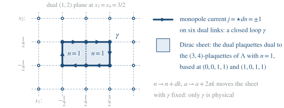
Figure 1. A monopole worldloop in four dimensions and its Dirac sheet: the Villain integer $n=1$ on two $(3,4)$-plaquettes of Λ is, on ${\Lambda }^{\ast }$, a sheet of two dual plaquettes whose boundary is the six-link loop $j=\star dn$ of Week 8 §5.5.

3. Energy against entropy

3.1 The action of one loop [Computed. The terms with $m\ge 3$ are a numerical estimate, reproducible from the stated protocol.]

Consider a single closed loop γ of $L$ unit links ${\ell }_1,\dots ,{\ell }_L$. Link ${\ell }_a$ lies along the axis ${\mu }_a$ with orientation $s_a=\pm 1$ and is based at the dual site $x_a$ from which it points in the $+{\mu }_a$ direction. Only parallel components interact, so

$$S[\gamma ]=2{\pi }^2\beta \sum _{\mu }⟨j_{\mu },G{j}_{\mu }⟩=2{\pi }^{2}G(0)\beta L+4{\pi }^2\beta \sum _{\begin{array}{c}a<b\\ {\mu }_a={\mu }_b\end{array}}{s}_a{s}_{b}G(x_a-x_b),$$

where the factor 4 counts each unordered pair twice. The lattice values follow from $G(x)={\int }_0^{\infty }dt{e}^{-8t}{\prod }_{\mu }{I}_{x_{\mu }}(2t)$, which is the Fourier form of conventions §2 after writing $1/{\hat{k}}^2={\int }_0^{\infty }dt{e}^{-t{\hat{k}}^2}$ and doing each momentum integral: $G(0)=0.154933$; $G(\hat{e})=G(0)-\frac{1}{8}=0.029933$ exactly, since $(\Delta G)(0)=8G(0)-8G(\hat{e})=1$; $G({\hat{e}}_1+{\hat{e}}_2)=0.012715$; $G(2{\hat{e}}_1)=0.008246$. Therefore the diagonal term is $3.058\beta$ per link, and the neighbours of a link contribute as follows:

• a straight step (two consecutive collinear links, same orientation): $+4{\pi }^{2}G(\hat{e})\beta =+1.182\beta$;
• a corner (consecutive perpendicular links): 0;
• a U-turn (links $a$ and $a+2$ antiparallel across one corner, at separation $\hat{e}$): $-1.182\beta$;
• links $a$ and $a+2$ parallel across one corner: $+4{\pi }^{2}G({\hat{e}}_1+{\hat{e}}_2)\beta =+0.502\beta$; collinear after two straight steps: $+4{\pi }^{2}G(2{\hat{e}}_1)\beta =+0.326\beta$.

For a random non-backtracking walk, which chooses each of the seven allowed continuations with probability $\frac{1}{7}$, the mean action per link is $2{\pi }^2\beta [G(0)+2{\sum }_{m\ge 1}\mathbb{E}(s_a{s}_{a+m}G(x_{a+m}-x_a)\left)\right]$, the expectation running over parallel pairs only. The $m=1$ term is $\frac{1}{7}(1.182)\beta =0.169\beta$. The $m=2$ term collects probability $\frac{1}{49}$ for two straight steps, $\frac{6}{49}$ for a corner followed by the original direction and $\frac{6}{49}$ for a U-turn:

$$\frac{0.326+6(0.502)-6(1.182)}{49}\beta =-0.077\beta .$$

The remaining terms are small and mostly negative; averaging them over $4\times 10^4$ sampled walks, up to $m=14$, gives $-0.07\beta$. Therefore

$$\bar{\epsilon }\beta \simeq (3.058+0.169-0.077-0.07)\beta =3.08\beta$$

per link, within about $0.01\beta$. The straight-step and U-turn corrections almost cancel, and the bare self-energy $3.06\beta$ is a good estimate of the cost of a crumpled loop. A straight worldline is much more expensive: Week 8 Problem 3 showed that a static monopole costs $2{\pi }^2{G}_3(0)\beta =4.99\beta$ per link, because every pair of its links is collinear.

3.2 Counting loops [Proved. for the bounds]

Let $c_L$ be the number of self-avoiding walks of $L$ steps from a fixed site of the hypercubic lattice in $d$ dimensions. A walk of $L+L^{\prime }$ steps is a walk of $L$ steps followed by one of $L^{\prime }$ steps, so $c_{L+L^{\prime }}\le c_L{c}_{L^{\prime }}$; the sequence $\ln c_L$ is subadditive, and the connectivity constant $\mu ={\lim }_{L\to \infty }{c}_L^{1/L}$ exists and equals ${\inf }_L{c}_L^{1/L}$. Walks that only step in positive directions are self-avoiding, and self-avoiding walks never backtrack, so

$$d^L\le c_L\le 2d(2d-1{)}^{L-1},\text{i.e.}d\le \mu \le 2d-1,$$

where the upper count is that of non-backtracking walks. In $d=4$, $4\le \mu \le 7$, and self-avoidance removes only the walks that close small circuits, so μ lies somewhat below 7. Two further facts enter the estimate without proof. Closing a walk into a loop costs a factor that grows more slowly than exponentially in $L$ (for a random walk in four dimensions the return probability after $L$ steps falls like $L^{-2}$), so closed loops are counted with the same μ. And a loop that traverses a link twice in the same direction carries current 2 there, which costs four times the diagonal action, while two traversals in opposite directions cancel and leave the link empty; so at the couplings of interest the relevant entropy per link is $\ln \mu$ with μ slightly below 7.

3.3 The free energy per length and the transition [Heuristic.]

A loop of length $L$ through a given link thus has weight about ${\mu }^L{e}^{-\bar{\epsilon }\beta L}$, up to factors subexponential in $L$, and the free energy per unit length is

$$f(\beta )=\bar{\epsilon }\beta -\ln \mu .$$

(Within the walk model, Jensen’s inequality $⟨e^{-S}⟩\ge e^{-⟨S⟩}$ makes $\bar{\epsilon }\beta -\ln \mu$ an upper bound on the true free energy per length.) The length distribution of loops is $P(L)\propto e^{-f(\beta )L}{L}^{-\upsilon }$ for some power $\upsilon$. For $f>0$ it decays exponentially, the mean loop length is finite, and loops are dilute and small. For $f<0$ the weight grows with $L$ without bound: in a real ensemble the growth is cut off only by the interactions among loops and by the size of the system, and loops of every size are present. The loops condense at $f=0$,

$${\beta }_c\simeq \frac{\ln \mu }{\bar{\epsilon }}=\frac{1.946}{3.06\text{to}3.08}=0.63\text{–}0.64(\mu =7),$$

and a value of μ below 7 lowers it slightly. Condensation occurs at small β, strong coupling, where the action per link is small; this is the confining side, consistent with the strong-coupling area law of Week 6. The estimate treats one loop at a time. It ignores the interactions between different loops, which in the dense phase screen the Coulomb self-energy and lower the cost of long loops, and it ignores the corrections to the counting of §3.2. It locates the transition; it does not prove that there is one, and it cannot tell its order (F1).

For comparison with Monte Carlo, the most precise determination is for the Wilson action: a first-order transition at ${\beta }_T=1.0111331(21)$ [Stated — refs: Arnold, Bunk, Lippert, Schilling 2003]. The Villain action is a different lattice model, and the standard way to compare the two is Villain’s matching of the fundamental character coefficient (conventions §4), $e^{-1/2{\beta }_V}=I_1({\beta }_W)/I_0({\beta }_W)$. At ${\beta }_W=1.0111331$ this gives $I_1/I_0=0.4503$ and ${\beta }_V=0.627$. The matching is itself approximate: for the two-dimensional XY model it maps the cosine critical coupling $1.12$ to $0.70$, while the Villain value is $0.75$ (conventions §5). Thus the agreement between $0.63$ and $0.627$ is better than either argument can justify, and we record it as a consistency check. Figure 2 collects the phase structure.

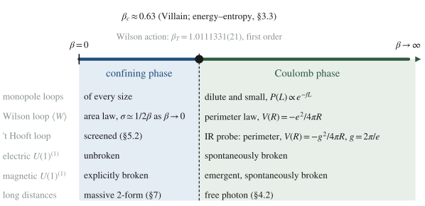
Figure 2. The phase diagram of four-dimensional Villain compact QED along β (schematic), with the realization of the two 1-form symmetries in each phase (Table 1) and the heuristic location of the transition; σ ≃ 1/2β is the leading strong-coupling tension of the Villain weight $e^{-b^2/2\beta }$ (Week 8 §3).

4. What a Wilson loop sees, and Guth’s theorem

4.1 The Wilson loop in the loop gas [Computed.]

The four-dimensional version of Week 8 Problem 1 shows how monopole loops act on a Wilson loop. Insert $W_q(C)=e^{iq⟨J_C,a⟩}$ with $q\in \mathbb{Z}$. Move 3 of Week 8 now imposes $\delta b=-q{J}_C$. With Σ a 2-chain of Λ bounded by $C$ and $\delta 1_{\Sigma }=J_C$ (Week 8 §2.2), the flux $b+q{1}_{\Sigma }$ is closed, and Week 8 §5.1 gives $b=\star (d\tilde{N}+w\cdot \tilde{M})-q{1}_{\Sigma }$. On the infinite lattice ($w=0$) the weight is $\exp (-\frac{1}{2\beta }\Vert d\tilde{N}-qX{\Vert }^2)$ with $X=\star 1_{\Sigma }\in C^2({\Lambda }^{\ast },\mathbb{Z})$, and the second Poisson resummation of Week 8 §5.2 replaces $\tilde{N}$ by the real field $\tilde{A}$ with the source $e^{2\pi i⟨j,\tilde{A}⟩}$. Split $X=X_{\mathrm{ex}}+X_{\mathrm{co}}$ into exact and coexact parts, with $X_{\mathrm{ex}}=d\psi$ and $\psi ={\Delta }^{-1}\delta X$. The shift $\tilde{A}\to \tilde{A}+q\psi$ removes $X_{\mathrm{ex}}$ from the action and moves it into the source; since $d\tilde{A}$ is exact and $X_{\mathrm{co}}$ coexact, the cross term vanishes, $\Vert d\tilde{A}-q{X}_{\mathrm{co}}{\Vert }^2=\Vert d\tilde{A}{\Vert }^2+q^2\Vert X_{\mathrm{co}}{\Vert }^2$, and the Gaussian integral over $\tilde{A}$ is that of Week 8 §5.5. Therefore

$$⟨W_q(C)⟩=\exp (-\frac{q^2}{2\beta }\Vert X_{\mathrm{co}}{\Vert }^2)⟨e^{2\pi iq⟨j,\psi ⟩}{⟩}_{\mathrm{loops}},\Vert X_{\mathrm{co}}{\Vert }^2=⟨J_C,G{J}_C⟩,$$

where the average is over the loop gas of §2. The second equality holds because $X_{\mathrm{co}}=\delta {\Delta }^{-1}dX$, so that $\Vert X_{\mathrm{co}}{\Vert }^2=⟨dX,{\Delta }^{-1}dX⟩$, while $dX=\pm \star J_C$ by the relation $\delta =\pm \star d\star$ of conventions §2, and ⋆ is an isometry that intertwines the Laplacians. The prefactor is the Wilson loop of the noncompact theory, $e^{-\frac{q^2{e}^2}{2}⟨J_C,G{J}_C⟩}$ with $\beta =1/e^2$: a perimeter law plus the Coulomb potential $V(R)=-q^2{e}^2/4\pi R$.

The phase contributed by a unit loop γ, bounded by a dual 2-chain σ with $J_{\gamma }=\delta 1_{\sigma }$, is

$$⟨J_{\gamma },\psi ⟩=⟨1_{\sigma },d{\Delta }^{-1}\delta X⟩=⟨1_{\sigma },X⟩-⟨1_{\sigma },X_{\mathrm{co}}⟩\equiv -\Omega (\gamma ,C)(\mathrm{mod}1),$$

where $⟨1_{\sigma },X⟩$ is an integer, the intersection number of the sheet of γ with Σ, which drops out of $e^{2\pi iq⟨j,\psi ⟩}$ because $q$ is an integer: Dirac quantization once more. Changing σ or Σ with fixed boundaries changes $\Omega =⟨1_{\sigma },X_{\mathrm{co}}⟩$ by an integer (for instance $\sigma \to \sigma +\partial V$ changes it by $⟨1_V,dX⟩=\pm \#(C\cap V)$), so $e^{-2\pi iq\Omega }$ depends only on the two loops. In four dimensions two loops have no topological linking, and Ω is a smooth function of their positions: the flux, through a sheet of γ, of the coexact field $X_{\mathrm{co}}$ that the Wilson loop sources. For a straight segment of $C$ that field falls like the field of a point charge in the three transverse dimensions, $|X_{\mathrm{co}}|\sim 1/4\pi {\rho }^2$ at distance ρ.

The dilute small-loop estimate [Heuristic.]. For a dilute gas of independent loops, $⟨e^{-2\pi iq{\sum }_{\gamma }{\Omega }_{\gamma }}⟩\simeq \exp [-{\sum }_{\gamma }{z}_{\gamma }(1-\cos 2\pi q\Omega (\gamma ,C)\left)\right]$, with $z_{\gamma }$ the weight of γ; the imaginary part cancels between γ and its reverse. A small loop of area $a^2$ at distance ρ from $C$ has $\Omega \sim a^2/4\pi {\rho }^2$, so $1-\cos 2\pi q\Omega \sim q^2{a}^4/8{\rho }^4$. Summed over positions at density $n$, the contribution per unit length of $C$ is $\int d^3\rho n{q}^2{a}^4/8{\rho }^4=\frac{\pi }{2}n{q}^2{a}^4{\int }_{{\rho }_0}^{\infty }d\rho /{\rho }^2$, which is finite and therefore scales like the perimeter. Small loops are magnetic dipoles, and dipoles produce only perimeter laws. A loop of linear size $r$ gives phases of order one only to Wilson loops of size $R\lesssim r$, so an area law for large $R$ requires loops of every size: the condensed phase of §3.3. In three dimensions the same formula has Ω equal to the solid angle of $C$ seen from a point monopole divided by $4\pi$, which is of order one for every monopole near the minimal surface, and a dilute plasma already gives the area law of Week 10.

4.2 Guth’s theorem and Fröhlich–Spencer [Stated — refs.], with a model bound [Proved.]

Theorem [Stated — refs: Guth 1980]. For four-dimensional $U(1)$ lattice gauge theory with the Villain action, the expectation value of the Wilson loop obeys a rigorous lower bound that, for sufficiently weak coupling (an explicit bound is given in the paper), has the form of the Coulomb interaction; static electric charges are therefore not confined. Together with the strong-coupling area law, which is a theorem for small β [Stated — refs: Osterwalder–Seiler 1978, as in Week 5], this proves that the model has at least one phase transition.

Theorem [Stated — refs: Fröhlich–Spencer 1982]. The deconfining transition is to a massless (QED) phase: at weak coupling the photon of four-dimensional $U(1)$ lattice gauge theory stays massless. Their method extends to the XY model in three or more dimensions and to abelian Higgs models.

Neither theorem says where the transition is, whether it is unique, or what its order is; those are the questions of §3.3 and F1. The proofs control the loop gas of §2 at large β, and the mechanism they make rigorous is the dipole estimate of §4.1.

A model bound [Proved.]. The first step of any such argument is that monopoles are rare at weak coupling, and a crude version is elementary. By Week 8 F7, $⟨F_P^2⟩=\frac{1}{\beta }-\frac{⟨b_P^2⟩}{{\beta }^2}\le \frac{1}{\beta }$ for the Villain field strength $F=da-2\pi n$, because the dual average of $b_P^2$ has positive weights. A cube with $m_c\ne 0$ has ${\sum }_{P\in \partial c}\pm F_P=-2\pi m_c$, so at least one of its six faces has $|F_P|\ge \pi /3$, and Chebyshev’s inequality gives

$$\mathrm{Prob}(m_c\ne 0)\le 6\cdot \frac{⟨F_P^2⟩}{(\pi /3{)}^2}\le \frac{54}{{\pi }^2\beta }=\frac{5.47}{\beta }.$$

The bound holds in $d=3$ as well, where the theory confines at every β. Monopoles thus become rare at weak coupling in both dimensions, and the difference between $d=3$ and $d=4$ lies in the geometry of §4.1.

Physical picture. A Monte Carlo simulation of the Villain model that records the monopole currents $j=\star dn$ sees, at large β, a dust of short loops, most of them the six-link loops of Figure 1 and their neighbours, and, below ${\beta }_c$, a tangle that spans the lattice. The Wilson loop tells the two apart for the reason of §4.1: a small loop acts on a distant Wilson loop as a dipole, with a phase that falls like $1/{\rho }^2$ and a cost that adds up to a perimeter, while a loop larger than the Wilson loop can wind around it with phases of order one. The exact statement is the formula for $⟨W_q(C)⟩$; the dipole counting is heuristic, and Guth’s theorem is the rigorous version at weak coupling. In three dimensions, where each monopole is a point charge with an order-one solid-angle phase, no such threshold exists.

5. The ‘t Hooft loop and the two 1-form symmetries

5.1 Twisted sheets and the electric symmetry [Proved.]

Consider a dual 2-chain $\tilde{S}$ on ${\Lambda }^{\ast }$ and let $\Xi ={\star }^{-1}{1}_{\tilde{S}}\in C^2(\Lambda ,\mathbb{Z})$ be the signed indicator of the plaquettes of Λ dual to its 2-cells (in $d=4$ plaquettes and dual plaquettes are dual to each other). For $\alpha \in \mathbb{R}$ define the twisted sheet $T_{\alpha }(\tilde{S})$ by replacing the Villain field strength $da-2\pi n$ with $da-2\pi n-\alpha \Xi$ in the weight and dividing by $Z$, keeping any other insertions. This is the $U(1)$ version of the flipped plaquettes of Week 5 §8 and conventions §6.

If $\tilde{S}=\partial \tilde{V}$ is closed, then $1_{\tilde{S}}=\delta 1_{\tilde{V}}$ on ${\Lambda }^{\ast }$, and the relation $\delta =\pm \star d\star$ of conventions §2 turns this into $\Xi =d\lambda$, where $\lambda \in C^1(\Lambda ,\mathbb{Z})$ is, up to the overall shuffle sign, the indicator of the links dual to the 3-cells of $\tilde{V}$. The substitution $a=a^{\prime }+\alpha \lambda$ preserves the measure over one period (the integrand is $2\pi$-periodic in each $a_{\ell }$) and removes the twist, $da-\alpha d\lambda =d{a}^{\prime }$, while $W_q(C)\to e^{iq\alpha ⟨J_C,\lambda ⟩}{W}_q(C)$. The integer $⟨J_C,\lambda ⟩$ counts, with signs, the links of $C$ dual to cells of $\tilde{V}$: it is the intersection number of $C$ with a 3-chain bounded by $\tilde{S}$, the linking number $\mathrm{Link}(C,\tilde{S})$ of a loop and a closed surface in four dimensions. Therefore, in every phase,

$$\boxed{⟨T_{\alpha }(\tilde{S})⟩=1,⟨T_{\alpha }(\tilde{S})W_q(C)⟩=e^{iq\alpha \mathrm{Link}(C,\tilde{S})}⟨W_q(C)⟩(\partial \tilde{S}=0).}$$

The closed twisted sheet is the symmetry operator $U_{\alpha }(\tilde{S})$ of the electric $U(1{)}^{(1)}$: its support is a closed 2-surface, as a 1-form symmetry requires in $d=4$ ($d-q-1=2$), and it acts on Wilson lines by linking (form-degree table, conventions §6; higher-form-symmetries).

5.2 The ‘t Hooft loop of compact QED is screened [Proved.]

Now let $\partial \tilde{S}=\tilde{C}$ be a dual loop and $\alpha =2\pi m$ with $m\in \mathbb{Z}$. The twisted field strength $da-2\pi (n+m\Xi )$ violates the Bianchi identity along $\tilde{C}$: its monopole current is $j+m\star d\Xi$, with $\star d\Xi =\pm J_{\tilde{C}}$, so $T_{2\pi m}(\tilde{S})$ forces a monopole worldline of charge $m$ along $\tilde{C}$ with Dirac sheet $\tilde{S}$. This is the ‘t Hooft loop ${\tilde{W}}_m(\tilde{C})$. But the twist is the relabeling $n\to n+m\Xi$ of the summed integers, so for every function $\mathcal{O}[a]$ of the gauge field

$$⟨{\tilde{W}}_m(\tilde{C})\mathcal{O}[a]⟩=⟨\mathcal{O}[a]⟩,\text{in particular}⟨{\tilde{W}}_m(\tilde{C})⟩=1.$$

In the loop gas the same statement reads $j\to j+m{J}_{\tilde{C}}$, absorbed by the sum over all conserved $j$. The Wilson action gives the same result, since it is $2\pi$-periodic in each plaquette angle. Thus the dynamical monopoles of compact QED screen every integer ‘t Hooft loop completely: the line can end on monopole operators, it is not the charged object of an exact symmetry, and it obeys a perimeter law (here with zero coefficient) in every phase. This is the lattice content of the entry “dynamical monopoles break it explicitly” for the magnetic $(d-3)$-form symmetry of the form-degree table, with $d-3=1$.

Two refinements make the table precise. In the Coulomb phase the loops are small, the explicit breaking is irrelevant at long distances, and the long-distance theory is free Maxwell theory with an emergent magnetic $U(1{)}^{(1)}$. Its ‘t Hooft line is a static monopole with its Coulomb field; it obeys a perimeter law with the magnetic Coulomb potential $V(R)=-g^2/4\pi R$, $g=2\pi /e$ (Week 8 Problem 3), so the emergent symmetry is spontaneously broken, with the photon as the Goldstone boson of both 1-form symmetries. We call this line the IR probe. It and the lattice loop ${\tilde{W}}_m=1$ are different operators, since no local counterterm produces a $1/R$ potential. The lattice loop is in effect the probe bound to a coincident dynamical anti-loop, which the sum over the Villain integers always supplies, and the line with the Coulomb potential exists only as a probe that the Villain sum cannot relabel, such as the genuine ‘t Hooft line of the monopole-free theory described next or an external static monopole source. And in the monopole-free Villain theory, where $dn=0$ is imposed (Semester II Week 12), the shift $n\to n+m\Xi$ violates the constraint, the relabeling fails, and the ‘t Hooft loop becomes a genuine line operator: by Week 8 §6 it is the Wilson loop of the dual photon at $\tilde{\beta }=1/4{\pi }^2\beta$.

5.3 The equal-time algebra [Proved.]

The commutation relation of Wilson and ‘t Hooft loops lives in the Hamiltonian slice of the four-dimensional theory, whose space has three dimensions, so that loops can link loops. Take the Kogut–Susskind Hamiltonian of Week 7, $H=\frac{g^2}{2}{\sum }_{\ell }{E}_{\ell }^2-\frac{1}{g^2}{\sum }_P\cos {\theta }_P$ with $E_{\ell }\in \mathbb{Z}$, $[E_{\ell },U_{{\ell }^{\prime }}]={\delta }_{\ell {\ell }^{\prime }}{U}_{\ell }$ and Gauss’s law $\delta E=-q$ (conventions §4). For a spatial dual surface $\tilde{S}$ define the electric flux ${\Phi }_E(\tilde{S})={\sum }_{\ell }{ϵ}_{\ell }{E}_{\ell }$, where ${ϵ}_{\ell }=\pm 1$ on the links pierced by $\tilde{S}$ (with the orientation of ℓ relative to $\tilde{S}$) and 0 elsewhere, and set

$${\tilde{W}}_{\alpha }(\tilde{C})=e^{i\alpha {\Phi }_E(\tilde{S})},\partial \tilde{S}=\tilde{C}.$$

Three properties follow. (i) For a closed surface, ${\Phi }_E(\partial V)$ is the outward flux, equal by Gauss’s law to the charge enclosed, which vanishes on the physical states of the pure gauge theory; so ${\tilde{W}}_{\alpha }$ depends only on $\tilde{C}$, and on a closed surface it is the electric symmetry operator, which acts as the identity there. (ii) Since $e^{i\alpha E}U{e}^{-i\alpha E}=e^{i\alpha }U$ on each link, ${\tilde{W}}_{\alpha }$ shifts ${\theta }_{\ell }\to {\theta }_{\ell }+\alpha {ϵ}_{\ell }$ on the pierced links, so every plaquette whose boundary crosses $\tilde{S}$ once, that is, every plaquette pierced by $\tilde{C}$, acquires magnetic flux $\pm \alpha$: ${\tilde{W}}_{\alpha }$ creates a thin tube of magnetic flux α along $\tilde{C}$. (iii) For a spatial Wilson loop $W_q(C)={\prod }_{\ell \in C}{U}_{\ell }^q$,

$$\boxed{{\tilde{W}}_{\alpha }(\tilde{C})W_q(C)=e^{iq\alpha \mathrm{Link}(C,\tilde{C})}{W}_q(C){\tilde{W}}_{\alpha }(\tilde{C}),}$$

because the oriented number of links of $C$ pierced by $\tilde{S}$ is the intersection number of $C$ with $\tilde{S}$, which in three dimensions is the linking number of $C$ with $\partial \tilde{S}$. This is the algebra of Wilson lines with the electric 1-form symmetry, the seed of Semester II Block 1, in its four-dimensional home; in three dimensions the magnetic symmetry is a 0-form symmetry with local charged operators (erratum E1, conventions §6).

At $\alpha =2\pi$ the operator is the identity, because $E_{\ell }$ is an integer: a flux tube of $2\pi$ is a Dirac string, invisible to every Wilson loop. That is the operator form of §5.2 and of Dirac quantization, and it is why the genuine ‘t Hooft loop of compact QED commutes with every Wilson loop. For $\alpha \notin 2\pi \mathbb{Z}$, ${\tilde{W}}_{\alpha }$ is the boundary of an electric symmetry surface, which Wilson lines detect, and in spacetime it is not a genuine line operator. In ${\mathbb{Z}}_N$ gauge theory, where $E_{\ell }\in {\mathbb{Z}}_N$, the choice $\alpha =2\pi /N$ gives the minimal ‘t Hooft loop, with $\tilde{W}W={\omega }^{q\mathrm{Link}}W\tilde{W}$, ‘t Hooft’s relation; on the physical states it depends only on $\tilde{C}$, but in spacetime it bounds the electric symmetry surface, which Wilson lines detect, so it is not a genuine line operator either; $N=2$ is Week 5 §8.3.

5.4 The phases and their symmetries

Table 1 collects the realization of the two 1-form symmetries by the SSB criterion of conventions §6 (a perimeter law for the charged loop means spontaneously broken, an area law unbroken), with the Higgs phase of a theory with charge-one electric matter and no monopoles added for contrast; that phase belongs to Week 13 and to §7.6.

	Coulomb phase (large β)	confining phase (small β)	Higgs phase (charge-1 matter, no monopoles)
Wilson loop $W_q$	perimeter, $V=-q^2{e}^2/4\pi R$	area	perimeter (screened)
‘t Hooft probe	IR probe: perimeter, $V=-m^2{g}^2/4\pi R$; lattice ${\tilde{W}}_m=1$, a different operator (§5.2)	perimeter (screened); lattice ${\tilde{W}}_m=1$	area (monopoles bound by flux tubes)
electric $U(1{)}^{(1)}$	spontaneously broken	unbroken	explicitly broken by the matter
magnetic $U(1{)}^{(1)}$	explicitly broken; emergent and spontaneously broken	explicitly broken	exact and unbroken
long-distance theory	free photon (Fröhlich–Spencer)	massive 2-form (§7)	massive photon, BF or Proca (§7.6)

Table 1. Loops and 1-form symmetries in the phases of four-dimensional abelian gauge theory. Only the Wilson loop distinguishes the two phases of compact QED; the magnetic symmetry is explicitly broken in both, and its emergence in the Coulomb phase is a long-distance statement.

6. The dual superconductor

6.1 An exact statement [Proved.]

For $\kappa >0$ consider on ${\Lambda }^{\ast }$ the dual photon $\tilde{a}\in C^1({\Lambda }^{\ast })$ with the monopole-free Villain action at $\tilde{\beta }=1/4{\pi }^2\beta$ of Week 8 §6, coupled to a charge-one compact scalar $\theta \in C^0({\Lambda }^{\ast })$ with Villain hopping κ:

$$Z_H(\tilde{\beta },\kappa )=\prod _{\tilde{\ell }}{\int }_{-\pi }^{\pi }\frac{d{\tilde{a}}_{\tilde{\ell }}}{2\pi }\prod _{\tilde{x}}{\int }_{-\pi }^{\pi }\frac{d{\theta }_{\tilde{x}}}{2\pi }\sum _{\begin{array}{c}\tilde{n}\in C^2({\Lambda }^{\ast },\mathbb{Z})\\ d\tilde{n}=0\end{array}}\sum _{k\in C^1({\Lambda }^{\ast },\mathbb{Z})}\exp (-\frac{\tilde{\beta }}{2}\Vert d\tilde{a}-2\pi \tilde{n}{\Vert }^2-\frac{\kappa }{2}\Vert d\theta -\tilde{a}-2\pi k{\Vert }^2).$$

The Villain identity of conventions §3 on each dual link, ${\sum }_k{e}^{-\frac{\kappa }{2}(u-2\pi k{)}^2}=(2\pi \kappa {)}^{-1/2}{\sum }_{l\in \mathbb{Z}}{e}^{-l^2/2\kappa +ilu}$ with $u=d\theta -\tilde{a}$, and the θ integrals, $\int \frac{d\theta }{2\pi }{e}^{i⟨\delta l,\theta ⟩}={\delta }_{\delta l,0}$, give

$$(2\pi \kappa {)}^{N_1^{\ast }/2}{Z}_H(\tilde{\beta },\kappa )=\sum _{\begin{array}{c}l\in C^1({\Lambda }^{\ast },\mathbb{Z})\\ \delta l=0\end{array}}{e}^{-\Vert l{\Vert }^2/2\kappa }{\tilde{Z}}_{\tilde{\beta }}[l],$$

where $N_1^{\ast }$ is the number of dual links and ${\tilde{Z}}_{\tilde{\beta }}[l]$ is the monopole-free theory with the source $e^{-i⟨l,\tilde{a}⟩}$ of Week 8 §6. Since ${\tilde{Z}}_{\tilde{\beta }}[l]$ vanishes unless $\delta l=0$ (gauge invariance), the identity of Week 8 §6 becomes

$$\boxed{Z_{\beta }=(2\pi \beta {)}^{-N_P/2}\underset{\kappa \to \infty }{\lim }(2\pi \kappa {)}^{N_1^{\ast }/2}{Z}_H(\frac{1}{4{\pi }^2\beta },\kappa ).}$$

At finite κ the same steps show that $(2\pi \beta {)}^{-N_P/2}(2\pi \kappa {)}^{N_1^{\ast }/2}{Z}_H$ is compact QED with the extra monopole weight $e^{-\Vert dn{\Vert }^2/2\kappa }$, because the source argument of Week 8 §5.3 identifies $l$ with $j=\star dn$ and $\Vert j{\Vert }^2=\Vert dn{\Vert }^2$ (a special case of the self-dual structure of Week 8 Problem 6⋆⋆).

The monopole loops are therefore the worldlines, in the current representation, of the charged scalar θ of the dual photon: the dual Higgs field. Its stiffness κ is the inverse of the core action per unit of monopole current, and pure Villain compact QED is the London limit $\kappa =\infty$, in which a monopole costs nothing beyond its Coulomb energy. At $\kappa =\infty$ the dual photon is frozen to a pure gauge modulo $2\pi$, and what remains are the closed integer surfaces $\tilde{n}$, which are the electric flux surfaces $\star b$ of Week 8 §3. When they are dilute (small β) the dual field is in its Higgs phase: the monopole condensate. When they proliferate (large β) the condensate is destroyed and the original photon is massless. For compact QED the dual superconductor of Nambu, ‘t Hooft and Mandelstam is thus an identity. What the identity does not contain is a radial mode for the dual Higgs field, which the continuum model of §6.2 adds, and any statement about where the Higgs phase lies, which is the business of §§3–4.

Physical picture. A superconductor expels magnetic flux because the phase of its condensate is stiff, and the London limit keeps only that phase. The identity above says that compact QED is a London superconductor for magnetic charge at infinite stiffness, with the electric flux surfaces of Week 8 §3 as its vortex sheets. A lattice simulation would see the electric flux of a static pair either spread in all directions (Coulomb phase, sheets proliferated) or confined to one sheet of minimal area (confining phase, sheets dilute), which is the dual Meissner effect. The identity is exact; the Ginzburg–Landau model of §6.2 is a model of it, and for QCD the whole picture is a hypothesis (F4).

6.2 The dual Ginzburg–Landau model and its vortex [Computed.; the model itself is Heuristic.]

The continuum model of the dual superconductor adds a radial mode to the London model. Its Euclidean action is

$$S_{\mathrm{dGL}}=\int d^{4}x[\frac{1}{4{\tilde{e}}^2}{\tilde{F}}_{\mu \nu }{\tilde{F}}_{\mu \nu }+|{\tilde{D}}_{\mu }\varphi {|}^2+\frac{\lambda }{4}(|\varphi {|}^2-v^2{)}^2],{\tilde{D}}_{\mu }={\partial }_{\mu }-i{\tilde{a}}_{\mu },\tilde{e}=\frac{2\pi }{e},$$

where φ is the monopole field of magnetic charge one, $v$ has mass dimension one, λ and $\tilde{e}$ are dimensionless, and $\frac{1}{4{\tilde{e}}^2}=\frac{e^2}{16{\pi }^2}$ is the dual Maxwell normalization of Week 8 §5.4. Around $\varphi =v$ the dual photon acquires its Meissner mass and the radial mode its own mass,

$$m_V^2=2{\tilde{e}}^2{v}^2,m_H^2=\lambda v^2,$$

with penetration depth ${\lambda }_L=1/m_V$ and core size $\xi =1/m_H$. The Bogomolny point $m_H=m_V$ separates type I ($m_H<m_V$) from type II ($m_H>m_V$); in the Ginzburg–Landau convention it is ${\kappa }_{\mathrm{GL}}=1/\sqrt{2}$.

The vortex. Consider a static tube along $x_3$, independent of $x_4$, with polar coordinates $(r,\vartheta )$ in the $(x_1,x_2)$ plane and the ansatz

$$\varphi =vf(r)e^{iq\vartheta },\tilde{a}=q\alpha (r)d\vartheta ,q\in \mathbb{Z},$$

so that ${\tilde{F}}_{12}=q{\alpha }^{\prime }/r$. Its action per unit area of the $(x_3,x_4)$ worldsheet, which is the tension, the energy per unit length of the static tube, is

$$T=2\pi {\int }_0^{\infty }rdr[\frac{q^2{\alpha }^{\prime 2}}{2{\tilde{e}}^2{r}^2}+v^2{f}^{\prime 2}+\frac{v^2{q}^2{f}^2(1-\alpha {)}^2}{r^2}+\frac{\lambda v^4}{4}(1-f^2{)}^2],$$

with $f(0)=\alpha (0)=0$ for regularity and $f(\infty )=\alpha (\infty )=1$ for finite tension. Varying $f$ and α gives the profile equations

$$f^{\prime \prime }+\frac{f^{\prime }}{r}-\frac{q^2(1-\alpha {)}^2}{r^2}f+\frac{m_H^2}{2}f(1-f^2)=0,{\alpha }^{\prime \prime }-\frac{{\alpha }^{\prime }}{r}+m_V^2{f}^2(1-\alpha )=0,$$

where the second comes from $\frac{d}{dr}\left(\frac{q^2{\alpha }^{\prime }}{{\tilde{e}}^{2}r}\right)=-\frac{2v^2{q}^2{f}^2(1-\alpha )}{r}$. Near the axis $f\propto r^{|q|}$ and $\alpha \propto r^2$; far away $1-\alpha \simeq m_{V}r{K}_1(m_{V}r)$ and $1-f$ decays like $K_0(m_{H}r)$ (for $m_H<2m_V$).

Dual flux quantization. Since $\tilde{a}\to qd\vartheta$ at infinity, $\int {\tilde{F}}_{12}{d}^{2}x={\oint }_{\infty }\tilde{a}=2\pi q$. The duality relation of Week 8 §5.4, $F\simeq \frac{i{e}^2}{2\pi }\star \tilde{F}$, with $\star \star =1$ on 2-forms, gives $\star F/e^2=\frac{i}{2\pi }\tilde{F}$, so the electric flux through the cross-section is $\int (\star F{)}_{12}/e^2=iq$: the tube carries $q$ units of electric flux along $x_3$, with the $i$ of Euclidean signature (F6). It is the flux tube of a charge-$q$ Wilson line.

The Bogomolny bound [Proved.]. With $D_j={\tilde{D}}_j$ and ${\epsilon }_{ij}\overline{D_i\varphi }{D}_j\varphi ={\epsilon }_{ij}{\partial }_i(\bar{\varphi }{D}_j\varphi )+i{\tilde{F}}_{12}|\varphi {|}^2$, which follows from $[D_1,D_2]=-i{\tilde{F}}_{12}$, one has

$$|D_1\varphi {|}^2+|D_2\varphi {|}^2=|(D_1+i{D}_2)\varphi {|}^2+{\tilde{F}}_{12}|\varphi {|}^2-i{\epsilon }_{ij}{\partial }_i(\bar{\varphi }{D}_j\varphi ),$$

and, writing ${\tilde{F}}_{12}|\varphi {|}^2={\tilde{F}}_{12}(|\varphi {|}^2-v^2)+v^2{\tilde{F}}_{12}$,

$$T=\int d^{2}x\left[\frac{1}{2{\tilde{e}}^2}\right({\tilde{F}}_{12}-{\tilde{e}}^2(v^2-|\varphi {|}^2){)}^2+|(D_1+i{D}_2)\varphi {|}^2+(\frac{\lambda }{4}-\frac{{\tilde{e}}^2}{2})(|\varphi {|}^2-v^2{)}^2]+v^2\int {\tilde{F}}_{12},$$

where the boundary term vanishes because $D\varphi \to 0$ exponentially. At $\lambda =2{\tilde{e}}^2$, that is $m_H=m_V$, the tension satisfies $T\ge 2\pi v^{2}q$ for $q>0$ (the other sign for $q<0$), with equality on the first-order equations $f^{\prime }=\frac{q}{r}(1-\alpha )f$ and $\frac{q{\alpha }^{\prime }}{r}=\frac{m_V^2}{2}(1-f^2)$. Therefore $T=2\pi v^2|q|$ at the Bogomolny point, and tubes of any charge neither attract nor repel there.

The type-II logarithm [Controlled to leading logarithm in $m_H/m_V$.]. For $\xi \ll r\ll {\lambda }_L$ we have $f\simeq 1$ and $\alpha \simeq 0$, and the gradient term $v^2{q}^2/r^2$ dominates the integrand, so

$$T\simeq 2\pi v^2{q}^2{\int }_{1/m_H}^{1/m_V}\frac{dr}{r}=2\pi v^2{q}^2\ln \frac{m_H}{m_V},$$

while the field and core terms contribute $O(v^2{q}^2)$ with no logarithm. Solving the profile equations numerically (a boundary-value solver on $10^{-4}\le m_{V}r\le 30$) gives, for $q=1$, $T/2\pi v^2=1.000$ at $m_H/m_V=1$, as the Bogomolny bound requires, and $1.961$, $2.540$, $3.180$, $3.852$ at $m_H/m_V=5$, 10, 20, 40, so that $T/2\pi v^2-\ln (m_H/m_V)=0.35$, 0.24, 0.18, 0.16 approaches a constant near 0.15. In type I the tension falls below the Bogomolny value, $T/2\pi v^2=0.757$ and $0.588$ at $m_H/m_V=0.5$ and $0.25$. In the original coupling, $v^2=m_V^2/2{\tilde{e}}^2=e^2{m}_V^2/8{\pi }^2$, and the unit tube has

$$T\simeq \frac{e^2{m}_V^2}{4\pi }[\ln \frac{m_H}{m_V}+O(1)].$$

Figure 3 shows the cross-section.

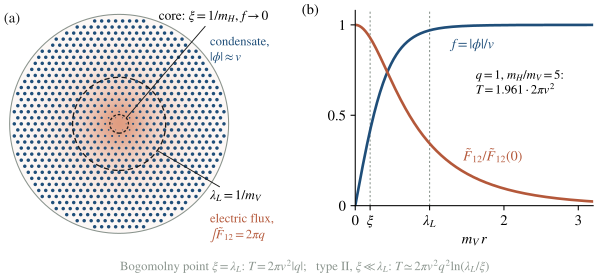
Figure 3. The dual Abrikosov tube, computed from the profile equations of §6.2 for $q=1$ at $m_H/m_V=5$, where $T/2\pi v^2=1.961$: (a) the cross-section, (b) the radial profiles. The monopole condensate (dots, $f=|\varphi |/v$) vanishes in a core of radius ξ, and the electric flux of a charge-$q$ Wilson line, $2\pi q$ in dual units (shading, ${\tilde{F}}_{12}=q{\alpha }^{\prime }/r$), is confined within the penetration depth ${\lambda }_L$.

6.3 The confining string [Heuristic.]

A static pair of charges $\pm q$ at separation $R\gg {\lambda }_L$ is joined by one such tube, and $V(R)\simeq TR$: the dual Meissner effect produces a linear potential. For compact QED the London limit of §6.1 is exact, and the tube is the sheet of minimal area of the electric flux surfaces of Week 8 §3; the radial mode and the values of $m_H$ and $m_V$ are model input. For QCD, the identification of the flux tube with a dual Abrikosov vortex is part of the dual-superconductor hypothesis discussed in F4.

7. The Julia–Toulouse mechanism

The dual superconductor answers what condenses. The Julia–Toulouse approach answers what the field content of the condensed phase is, directly in the variables of the original photon, and it is the form in which the group’s research line has used the idea since 2009. The answer is a change of rank: the integer Dirac sheets become a continuous 2-form and the photon disappears into it.

7.1 The exact starting point: Dirac sheets and their redundancy [Proved.]

The Villain weight depends on $n$ only through $da-2\pi n$, and the branch shift $n\to n+dk$, $a\to a+2\pi k$ ($k\in C^1(\Lambda ,\mathbb{Z})$) moves the Dirac sheets with their boundaries fixed (§2). Its invisibility to integer charges is Dirac quantization (Week 8 §2.2). In the group’s papers this redundancy is called the Dirac brane symmetry; it is a redundancy of the description, and Elitzur’s theorem forbids its spontaneous breaking in the literal sense (Week 5 §3). The sum over sheets can be written as an integral over a real 2-form with a comb measure,

$$\sum _{n\in C^2(\Lambda ,\mathbb{Z})}{e}^{-\frac{\beta }{2}\Vert da-2\pi n{\Vert }^2}=\int \prod _{P}d{L}_P{\rho }_{\mathrm{comb}}[L]e^{-\frac{\beta }{2}\Vert da-L{\Vert }^2},{\rho }_{\mathrm{comb}}[L]=\prod _P\sum _{n_P\in \mathbb{Z}}\delta (L_P-2\pi n_P)=\prod _P\frac{1}{2\pi }\sum _{b_P\in \mathbb{Z}}{e}^{i{b}_P{L}_P},$$

where the last form is Poisson’s identity (conventions §3): the Fourier modes of the comb are the integer electric fluxes $b$ of Week 8 §3. Everything so far is exact, and the only physical content of $L$ is its boundary, the monopole current $j=\star dL/2\pi$.

7.2 The prescription [Heuristic: the Julia–Toulouse prescription.]

In the Coulomb phase the loops are small, and each sheet can be chosen inside a region of the size of its loop: the sheets are sparse, and the comb, which forces them to be integer, is essential. When loops proliferate at every scale ($f<0$ in §3.3), the sheets fill space. On scales much longer than the lattice spacing the coarse-grained sheet density is a real 2-form Λ, whose only gauge-invariant content is the coarse-grained monopole current $j=\star d\Lambda /2\pi$. The Julia–Toulouse prescription replaces the comb by a smooth measure that depends on Λ only through that current, at the lowest order in derivatives,

$${\rho }_{\mathrm{comb}}[\Lambda ]⟶{\rho }_{\mathrm{JT}}[\Lambda ]\propto \exp (-\frac{1}{2g^2}\Vert d\Lambda {\Vert }^2),$$

and in the continuum, with $\beta =1/e^2$ in $d=4$, the effective theory of the condensed phase becomes

$$S_{\mathrm{JT}}[a,\Lambda ]=\int [\frac{1}{2e^2}(da-\Lambda )\wedge \star (da-\Lambda )+\frac{1}{2g^2}d\Lambda \wedge \star d\Lambda ],$$

where $g$ has mass dimension one and is a phenomenological parameter of the condensate, the counterpart of a London penetration length. The integer redundancy of §7.1 has become a continuous 1-form gauge redundancy,

$$a\to a+\xi ,\Lambda \to \Lambda +d\xi ,\xi \in {\Omega }^1\text{real},$$

of which the ordinary gauge transformations are the special case $\xi =d\chi$. The step from ${\rho }_{\mathrm{comb}}$ to ${\rho }_{\mathrm{JT}}$ is not derived here from the microscopic loop gas, and the sources treat it as a prescription. Three things support it. It is the lowest-order local measure compatible with the continuous redundancy, since any functional of Λ alone that is invariant under $\Lambda \to \Lambda +d\xi$ depends on $d\Lambda$ only. It is, by §7.4, the London limit of the exact dual Higgs theory of §6.1 with a finite effective stiffness. And it reproduces the loop laws of the confining phase (§7.5).

The prescription goes back to Julia and Toulouse (1979), who proposed it for ordered media containing defects. Quevedo and Trugenberger (1997) formulated it for compact antisymmetric tensors of rank $h-1$ in $D$ dimensions, with compact QED in four dimensions as their detailed example: starting from the Coulomb phase, the condensation of the topological defects leads to a generalized confinement phase, and each phase has two dual descriptions by antisymmetric tensors of different ranks, massless in the Coulomb phase and massive in the Higgs and confinement phases. In the formulation used by Grigorio, Guimaraes, Rougemont and Wotzasek in Phys. Lett. B 690 (2010) 316, once the magnetic strings of the monopoles proliferate everywhere, the observable field strength can no longer be written in terms of the gauge field, and the prescription takes it as the fundamental field of the condensed phase, supplemented by a kinetic term, which yields the massive Kalb–Ramond action. In the Villain variables the observable field strength is $da-2\pi n$, and in the gauge $a=0$ of §7.3 it is $-\Lambda$.

7.3 The rank change [Computed. within the prescription]

Choose $\xi =-a$. Then $a\to 0$ and, renaming $\Lambda -da$ as Λ,

$$S_{\mathrm{JT}}=\int [\frac{1}{2e^2}\Lambda \wedge \star \Lambda +\frac{1}{2g^2}d\Lambda \wedge \star d\Lambda ].$$

The field equation $\frac{1}{g^2}\delta d\Lambda +\frac{1}{e^2}\Lambda =0$ implies, after applying δ, $\delta \Lambda =0$, and therefore

$$(\Delta +m^2)\Lambda =0,\delta \Lambda =0,m^2=\frac{g^2}{e^2}.$$

A 2-form in four dimensions has six components; the four conditions $\delta \Lambda =0$ are related by $\delta \delta =0$ and remove three, so a massive 2-form carries three polarizations, the content of a massive vector. The Coulomb phase has one massless 1-form with two polarizations. The photon has been absorbed by the field of Dirac sheets, the extra polarization comes from the condensate (it is the phase θ of the dual Higgs field in §7.4), and the long-distance field of the confining phase is a massive 2-form. This change of rank is the Julia–Toulouse statement, the rank-jump of the group’s papers. It comes with a new gauge redundancy whose parameter is a 1-form; what that means in the language of higher-form symmetries, gauging and condensation defects is the subject of Semester II Week 14.

7.4 Three descriptions of one condensate [Computed. within the prescription; flux sectors and vortex sheets dropped]

(a) → (b): the BF form with the dual photon. Write the first term of $S_{\mathrm{JT}}$ with a Hubbard–Stratonovich 2-form $b$, $e^{-\frac{1}{2e^2}\Vert X{\Vert }^2}\propto \int Db{e}^{-\frac{e^2}{2}\Vert b{\Vert }^2+i⟨b,X⟩}$ with $X=da-\Lambda$, the continuum form of Move 1 of Week 8. The integral over $a$ imposes $\delta b=0$ (on ${\mathbb{R}}^4$, dropping flux sectors), solved as in Week 8 by $b=-\frac{1}{2\pi }\star d\tilde{a}$, where $\tilde{a}$ is the dual photon with the sign convention of Week 8 §5.4. Then $\frac{e^2}{2}\Vert b{\Vert }^2=\frac{e^2}{8{\pi }^2}\Vert d\tilde{a}{\Vert }^2=\frac{1}{2{\tilde{e}}^2}\Vert d\tilde{a}{\Vert }^2$, and, since $⟨\star d\tilde{a},\Lambda ⟩=\int \Lambda \wedge \star \star d\tilde{a}=\int \Lambda \wedge d\tilde{a}$ for 2-forms in four dimensions, $-i⟨b,\Lambda ⟩=\frac{i}{2\pi }\int \Lambda \wedge d\tilde{a}$. Therefore

$$S_{\mathrm{BF}}[\tilde{a},\Lambda ]=\int [\frac{1}{2{\tilde{e}}^2}d\tilde{a}\wedge \star d\tilde{a}+\frac{1}{2g^2}d\Lambda \wedge \star d\Lambda -\frac{i}{2\pi }\Lambda \wedge d\tilde{a}].$$

The 2-form couples at level one ($N=1$ in the normalization $\frac{iN}{2\pi }\int b\wedge da$ of conventions §7) to the dual photon. Integrating by parts, $\int \Lambda \wedge d\tilde{a}=-\int d\Lambda \wedge \tilde{a}$, and with $d\Lambda =-2\pi \star j$, which follows from $j=\star d\Lambda /2\pi$ and $\star \star =-1$ on 3-forms in four dimensions, this is the coupling $e^{-i⟨j,\tilde{a}⟩}$ of the monopole current to the dual photon found in Week 8 §5.4.

(b) → (c): the London form. Write the second term with a 3-form $Y$, $e^{-\frac{1}{2g^2}\Vert H{\Vert }^2}\propto \int DY{e}^{-\frac{g^2}{2}\Vert Y{\Vert }^2+i⟨Y,H⟩}$ with $H=d\Lambda$. Now Λ appears linearly, $i⟨\delta Y,\Lambda ⟩+\frac{i}{2\pi }⟨\Lambda ,\star d\tilde{a}⟩$, and its integral imposes $\delta Y=-\frac{1}{2\pi }\star d\tilde{a}$. With $\delta =-\star d\star$ on 3-forms and $\star \star =-1$ on 1-forms in four dimensions, the general solution is

$$Y=\frac{1}{2\pi }\star (d\theta -\tilde{a}),$$

with θ a scalar whose periodicity comes from the flux quantization of Λ, dropped here. Then $\frac{g^2}{2}\Vert Y{\Vert }^2=\frac{g^2}{8{\pi }^2}\Vert d\theta -\tilde{a}{\Vert }^2$ and

$$S_{\mathrm{L}}[\tilde{a},\theta ]=\int [\frac{1}{2{\tilde{e}}^2}d\tilde{a}\wedge \star d\tilde{a}+\frac{\kappa }{2}(d\theta -\tilde{a})\wedge \star (d\theta -\tilde{a})],\kappa =\frac{g^2}{4{\pi }^2}.$$

This is the London model of the dual superconductor, whose Meissner mass is $\kappa {\tilde{e}}^2=\frac{g^2}{4{\pi }^2}\cdot \frac{4{\pi }^2}{e^2}=\frac{g^2}{e^2}=m^2$, the mass of §7.3. Figure 4 assembles the three forms.

The Julia–Toulouse action is therefore the London limit of the dual superconductor at the finite stiffness $\kappa =g^2/4{\pi }^2$, with the vortex sheets of θ dropped. Those sheets are the electric flux tubes of §6.2; in the Higgs phase they are massive and appear only as strings attached to Wilson lines. Dropping them is the complete-condensation limit, and this is the content of Phys. Lett. B 690 (2010) in the course’s variables: there Grigorio, Guimaraes, Rougemont and Wotzasek compared the Julia–Toulouse approach with the approach built on the Banks–Myerson–Kogut lattice rewriting (and on Kleinert’s disorder-field theory), which they call ALBA, and showed with a generalized Poisson identity for branes that the two are dual-equivalent prescriptions in the limit where the Poisson-dual current vanishes, which characterizes complete condensation; a nonzero Poisson-dual current describes vortex-like defects in the condensate, the role the θ-sheets play here. The comparison with §6.1 contains one more lesson. The exact identity has bare stiffness $\kappa =\infty$, while the effective κ is finite: the virtual electric flux surfaces renormalize the stiffness, as vortex pairs renormalize the stiffness of the XY model in Week 4, and the prescription does not compute the result.

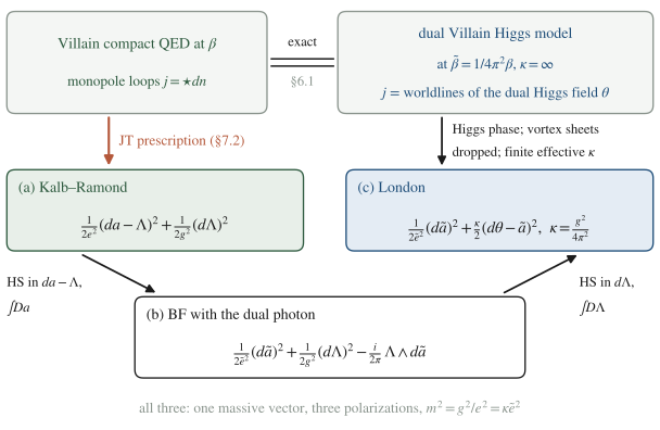
Figure 4. One condensate, three descriptions: the Julia–Toulouse form in the original variables (a), the level-one BF form with the dual photon (b) and the London form of the dual superconductor (c), related by Gaussian dualities; the exact identity of §6.1 sits above them at infinite bare stiffness.

7.5 Wilson and ‘t Hooft loops in the condensate [Computed. within the prescription]

Wilson loops need surfaces. Under the redundancy of §7.2 the phase ${\oint }_{C}a$ shifts by ${\oint }_C\xi$, so the bare Wilson line is not invariant; the invariant completion is

$$W(C,S)=\exp (i{\oint }_{C}a-i{\int }_S\Lambda ),\partial S=C,$$

because ${\int }_{S}d\xi ={\oint }_C\xi$. Every Wilson line of the condensed phase carries a surface. In the gauge $a=0$, $W=e^{-i⟨1_S,\Lambda ⟩}$, with $⟨1_S,\Lambda ⟩={\int }_S\Lambda$ and $\delta 1_S=J_C$ as in Week 8 §2.2. The action of §7.3 is $\frac{1}{2}⟨\Lambda ,K\Lambda ⟩$ with $K=\frac{1}{e^2}(1+\delta d/m^2)$. On exact 2-forms $\delta d=0$ and $K^{-1}=e^2$; on coexact 2-forms $\delta d=\Delta$ and $K^{-1}=e^2{m}^2/(m^2+\Delta )$. With the Hodge split $1_S=P_{\mathrm{ex}}{1}_S+P_{\mathrm{co}}{1}_S$ on ${\mathbb{R}}^4$ and $P_{\mathrm{ex}}{1}_S=d{\Delta }^{-1}\delta 1_S=d{\Delta }^{-1}{J}_C$,

$$\ln ⟨W(C,S)⟩=-\frac{e^2}{2}[\Vert P_{\mathrm{ex}}{1}_S{\Vert }^2+⟨P_{\mathrm{co}}{1}_S,\frac{m^2}{m^2+\Delta }{P}_{\mathrm{co}}{1}_S⟩]=-\frac{e^2}{2}⟨1_S,\frac{m^2}{m^2+\Delta }{1}_S⟩-\frac{e^2}{2}⟨P_{\mathrm{ex}}{1}_S,\frac{\Delta }{m^2+\Delta }{P}_{\mathrm{ex}}{1}_S⟩,$$

and the last term equals $⟨J_C,{\Delta }^{-1}\delta d(m^2+\Delta {)}^{-1}{J}_C⟩=⟨J_C,(m^2+\Delta {)}^{-1}{J}_C⟩$, because $\delta J_C=0$ gives $\delta d{J}_C=\Delta J_C$. Therefore

$$\boxed{\ln ⟨W(C,S)⟩=-\frac{e^2}{2}⟨1_S,\frac{m^2}{m^2+\Delta }{1}_S⟩-\frac{e^2}{2}⟨J_C,\frac{1}{m^2+\Delta }{J}_C⟩.}$$

The second term is the Yukawa self-energy of the loop, a perimeter term. The first is a surface term. For a large flat $S$ the kernel is evaluated at zero separation transverse to $S$ and integrated over the plane, which sets the momenta along $S$ to zero:

$$\sigma =\frac{e^2}{2}\int \frac{d^2{k}_{\perp }}{(2\pi {)}^2}\frac{m^2}{m^2+k_{\perp }^2}=\frac{e^2{m}^2}{8\pi }\ln (1+\frac{{\Lambda }_{\mathrm{UV}}^2}{m^2})\simeq \frac{e^2{m}^2}{4\pi }\ln \frac{{\Lambda }_{\mathrm{UV}}}{m}.$$

This is an area law. The logarithm is the type-II logarithm: the effective theory has no core, and its cutoff is the scale where it stops being valid, the core $\xi =1/m_H$ of the tube. With ${\Lambda }_{\mathrm{UV}}=m_H$ and $m=m_V$, $\sigma =\frac{e^2{m}_V^2}{4\pi }\ln \frac{m_H}{m_V}$, the London tension of §6.2 at leading logarithm. The dependence on $S$ is physical: $S$ is the worldsheet of the flux tube, and a Wilson line of the condensed phase is attached to it. In the language of JHEP 08 (2011) 118, the Dirac string has become part of a brane-invariant observable with energy content.

‘t Hooft loops are screened. A static external monopole on $\tilde{C}$ is an extra integer sheet Ξ bounded by $\tilde{C}$, $da-\Lambda \to da-\Lambda -2\pi \Xi$. The shift $\Lambda \to \Lambda -2\pi \Xi$ moves it into the kinetic term, $\frac{1}{2g^2}\Vert d\Lambda -2\pi d\Xi {\Vert }^2$, so only $d\Xi$ enters and the sheet is invisible. Completing the square in the gauge $a=0$, with $\delta d\Xi =\Delta {\Xi }_{\mathrm{co}}$ and $e^2{m}^2/g^4=1/g^2$,

$$\ln ⟨\tilde{W}(\tilde{C})⟩=-\frac{2{\pi }^2}{g^2}⟨{\Xi }_{\mathrm{co}},(\Delta -\frac{{\Delta }^2}{m^2+\Delta }){\Xi }_{\mathrm{co}}⟩=-\frac{2{\pi }^2}{e^2}⟨J_{\tilde{C}},\frac{1}{m^2+\Delta }{J}_{\tilde{C}}⟩,$$

where the last step uses ${\Xi }_{\mathrm{co}}=\delta {\Delta }^{-1}d\Xi$ and $d\Xi =\pm \star J_{\tilde{C}}$. This is a perimeter law with a Yukawa kernel: the magnetic charge $g_m=2\pi /e$ is screened by the condensate, as Table 1 requires. As $m\to 0$ the surface term vanishes and both kernels become Coulombic, $\ln ⟨W⟩\to -\frac{e^2}{2}⟨J_C,G{J}_C⟩$ and $\ln ⟨\tilde{W}⟩\to -\frac{g_m^2}{2}⟨J_{\tilde{C}},G{J}_{\tilde{C}}⟩$, the two perimeter laws of the Coulomb phase.

Physical picture. The rank change is visible in what probes can do. In the Coulomb phase a Wilson line is a line, and any Dirac string we attached to it would be invisible. In the condensed phase the Dirac sheets have become a field with its own dynamics, the line can exist only as the edge of a sheet of that field, and the sheet costs σ per unit area: confinement is the statement that the redundancy of the Dirac branes has become a gauge redundancy with a 1-form parameter, under which naked Wilson lines are not invariant. A static monopole, on the contrary, is the edge of a sheet that the condensate absorbs, and it is screened. All of this is exact within the Gaussian effective theory; the effective theory itself rests on the prescription of §7.2, and its parameter $m$ is not computed. This is the mechanism the group’s series studied from 2009 to 2013, and the modern re-reading of the same sheet ensemble, restricted to a hypersurface, is the subject of the group’s current work (condensation-defects).

7.6 The electric condensate and the group’s papers

Electric–magnetic duality (Week 8 §6) exchanges the monopoles of the original with the electric charges of the dual. If electric matter of the original condenses, the same prescription applied to the sheets bounded by the charged worldlines gives the Kalb–Ramond form for the dual photon, $\frac{1}{2{\tilde{e}}^2}(d\tilde{a}-{\Lambda }_e{)}^2+\frac{1}{2g_e^2}(d{\Lambda }_e{)}^2$, and §7.4 with $a\leftrightarrow \tilde{a}$ turns it into

$$S=\int [\frac{1}{2e^2}da\wedge \star da+\frac{1}{2g_e^2}dB\wedge \star dB-\frac{i}{2\pi }B\wedge da],$$

a level-one BF term with the original photon. In this phase Wilson lines are screened and a static monopole needs a surface, which carries a tension: the Higgs column of Table 1. Integrating out $B$ instead gives a Proca theory, a massive photon. The two condensates are distinguished by which loop needs a surface.

The group’s series, paper by paper:

• Grigorio, Guimaraes, Wotzasek, “Monopoles in the presence of the Chern–Simons term via the Julia–Toulouse approach”, Phys. Lett. B 674 (2009) 213 [0808.3698]: QED₃ with magnetic-like defects and a Chern–Simons term; the non-conserved electric current of the Maxwell–Chern–Simons–monopole system is interpreted as originating from the breaking of the Dirac brane symmetry, the low-energy effective theory gives the physical origin of the deconfinement transition, and the fermionic determinant is computed in the presence of Dirac branes.
• Grigorio, Guimaraes, Rougemont, Wotzasek, “Dual approaches for defects condensation”, Phys. Lett. B 690 (2010) 316 [0908.0370]: the equivalence of the Julia–Toulouse approach and ALBA in the limit of complete condensation, discussed in §7.4, with the monopole example in $3+1$ dimensions and the massive Kalb–Ramond action.
• Grigorio, Guimaraes, Rougemont, Wotzasek, “Confinement, brane symmetry and the Julia–Toulouse approach for condensation of defects”, JHEP 08 (2011) 118 [1102.3933]: proposes what the paper calls the spontaneous breaking of the brane symmetry as a universal criterion for charge confinement in abelian gauge theories, meaning that the Dirac string becomes part of a brane-invariant observable with energy content (the surface of §7.5), and generalizes the prescription to be compatible with Elitzur’s theorem and to condensates that break Lorentz and discrete spacetime symmetries.
• Grigorio, Guimaraes, Rougemont, Wotzasek, Zarro, “The BF theory as an electric Julia–Toulouse condensate”, Phys. Rev. D 86 (2012) 027705 [1202.3798]: the abelian BF term induced by the condensation of electric charges; magnetic defects included consistently in the Maxwell–BF theory; Dirac’s veto obtained from the Dirac brane symmetry.
• Guimaraes, Rougemont, Wotzasek, Zarro, “Massive photons and Dirac monopoles: electric condensate and magnetic confinement”, Phys. Lett. B 723 (2013) 422 [1209.3073]: the Proca theory as the effective theory of an electric condensate, whose Meissner effect confines magnetic defects into monopole–antimonopole pairs joined by physical open magnetic vortices described by Dirac-brane invariants.

The same authors’ Julia–Toulouse treatment of the bosonized Schwinger model is Phys. Rev. D 86 (2012) 125039 [1209.2751], which is why “PRD 86” alone is ambiguous (bibliography-and-paper-map).

7.7 Looking forward: the restricted sheet ensemble

The prescription of §7.2 keeps the integer sheets only through their continuous coarse-graining. Semester II Week 14 keeps integer variables of this kind. In $2+1$ dimensions it restricts charge-$k$ Villain matter to a surface, and in the London limit the restricted ensemble is the condensation sheet of higher gauging, whose field is $-k$ times the matter current reduced modulo $N$; in four dimensions the field of the higher-gauging wall is the restricted Villain integer reduced modulo $N$. The group’s manuscript in preparation studies the Wilson-line endpoints on such walls and gives the lines that join them a finite cost. That is the subject of Semester II Week 14 and of the master-project; nothing in this note depends on it.

8. Subtleties and fine print

F1 — Order and location of the transition. The energy–entropy balance of §3.3 cannot decide the order of the transition, and neither theorem of §4.2 addresses it. For the Wilson action, finite-size scaling of plaquette cumulants in the Borgs–Kotecký scheme gives a first-order transition at ${\beta }_T=1.0111331(21)$ [Stated — refs: Arnold, Bunk, Lippert, Schilling 2003]. That result is for the Wilson action; the Villain model, to which the loop-gas argument and Guth’s theorem apply, is a different lattice regularization. At a first-order transition the correlation length stays finite, so the transition point defines no continuum limit, and the continuum physics of the model is that of its two phases.

F2 — Monopole mass versus line tension. The Euclidean action per unit length of a straight worldline is the mass of a static monopole, $M{a}_{\mathrm{lat}}=4.99\beta$ (Week 8 Problem 3). The quantity that decides proliferation is the free energy per unit length of random loops, whose mean action is $\bar{\epsilon }\beta \simeq 3.08\beta$ per link (§3.1), because random loops are crumpled and collinear pairs are rare. Using the mass in the energy–entropy estimate would give ${\beta }_c\simeq \ln 7/4.99=0.39$, which is wrong. Near a first-order transition neither quantity vanishes.

F3 — Condensation is a statement about the distribution of loop lengths. “The loops condense” means that $P(L)$ stops decaying exponentially: in the confining phase a finite fraction of the monopole current belongs to loops as large as the system. The Wilson loop of size $R$ is sensitive only to loops of linear size $\gtrsim R$ (§4.1), so the area law and the proliferation of long loops are the same statement read in two ways. In the London form, the gauge-invariant two-point function of the dual Higgs field, $⟨e^{i\theta (x)}{e}^{-i{\int }_x^y\tilde{a}}{e}^{-i\theta (y)}⟩$, is in the current representation a sum over configurations with an open monopole line from $x$ to $y$. It decays exponentially when lines are short and tends to a constant when they proliferate, which is the gauge-invariant (and non-local) content of "$⟨\varphi ⟩\ne 0$" [Heuristic.].

F4 — Abelian projection and QCD. For $SU(N)$ there is no magnetic $U(1)$ to condense until a gauge is partially fixed. ‘t Hooft (1981) proposed fixing it up to the Cartan torus $U(1{)}^{N-1}$; the abelian gauge fields that remain carry monopoles at the points where the gauge condition is singular, and confinement would be their condensation. The monopoles, their density and the degree to which they dominate the string tension depend on the gauge condition; lattice studies commonly use the maximal abelian gauge, and the gauge-invariant content of the picture has not been settled. The dual superconductor is therefore a hypothesis for QCD, supported by gauge-dependent evidence. The controlled four-dimensional example of confinement by monopole condensation is $\mathcal{N}=2$ supersymmetric Yang–Mills theory with a mass term that breaks it to $\mathcal{N}=1$, where monopoles become light near a point of the moduli space and condense [Stated — refs: Seiberg–Witten 1994]. For compact QED the picture is an identity (§6.1).

F5 — What the prescription computes and what it does not. Within the Julia–Toulouse action the spectrum, the rank change, the area law and the screening of monopoles follow exactly (§§7.3–7.5). The parameter $g$, equivalently κ or $m$, is not computed: the exact identity of §6.1 fixes only the bare stiffness $\kappa =\infty$. The prescription also does not describe the transition itself, where the description changes discontinuously, and a partially condensed phase needs the vortex sheets that §7.4 dropped, the Poisson-dual current of Phys. Lett. B 690.

F6 — The Euclidean $i$ in the flux dictionary. In Euclidean variables $\star F/e^2=\frac{i}{2\pi }\tilde{F}$, so a real dual flux corresponds to an imaginary Euclidean electric field; statements about “electric flux in the tube” refer to the continuation to real time, as in Week 8 §5.4. The saddles of the dual Ginzburg–Landau model are real in the dual variables, which is one reason the dual description is the natural one for confinement.

F7 — Perimeter coefficients are scheme-dependent. On the Villain lattice the integer ‘t Hooft loop equals 1 identically (§5.2), while in the effective theory of §7.5, which describes the confining phase, a static monopole distinguished from the dynamical ones has a Yukawa perimeter term. Both are perimeter laws. A perimeter coefficient depends on how the probe is regularized and can be changed by a local counterterm; the dichotomy between area and perimeter laws cannot. This reconciliation covers only the confining column of Table 1. In the Coulomb phase the IR probe has the potential $-m^2{g}^2/4\pi R$, which no local counterterm produces, so it and the lattice loop are different operators (§5.2).

9. Common misconceptions

• “The dual superconductor has been proven for QCD.” It is tempting because for compact QED the statement is an exact identity (§6.1), and because lattice studies in the maximal abelian gauge report monopole condensation and abelian dominance. For $SU(N)$ the monopoles exist only after abelian projection, and their properties depend on the gauge condition (F4). The dual superconductor is a hypothesis for QCD; the controlled four-dimensional example is the softly broken $\mathcal{N}=2$ theory of Seiberg and Witten.
• “Monopole condensation means that a local monopole field acquires an expectation value.” It is tempting because the Ginzburg–Landau model of §6.2 is written with $⟨\varphi ⟩=v$. The field φ is charged under the dual gauge field, and by Elitzur’s theorem its expectation value vanishes in every gauge-invariant treatment. What condenses is an ensemble of closed worldlines, and its gauge-invariant signatures are non-local: the distribution of loop lengths, the endpoint correlator of an open monopole line (F3), and the Julia–Toulouse change of rank, in which the integer Dirac sheets become a continuous 2-form and Wilson lines acquire surfaces (§§7.3, 7.5).
• “The effective theory of monopole condensation is $B\wedge F$ with the original photon.” It is tempting because BF theories describe gapped phases of gauge fields. A level-one BF term with the original photon screens Wilson lines and confines monopoles: it is the electric condensate of Phys. Rev. D 86 (2012) 027705 (§7.6). The monopole condensate couples its 2-form to the dual photon, or, in the original variables, lets the 2-form absorb the photon; the test is which loop needs a surface.
• “In four dimensions, as in three, a dilute monopole gas confines.” It is tempting because Polyakov’s mechanism works at any density. A four-dimensional monopole is a loop, a small loop acts on a large Wilson loop as a dipole, and dipoles give a perimeter law (§4.1); an area law requires loops as large as the Wilson loop, which appear only when the entropy of long loops beats their action (§3.3).

10. Historical note

Nambu (1974) described monopoles joined by the vortex strings of a superconducting vacuum as a model of confined constituents, and ‘t Hooft, at the Palermo conference of 1975, and Mandelstam (1976) turned the picture around: if the vacuum of a gauge theory condenses magnetic monopoles, electric flux is squeezed into vortices and electric charges are confined. Banks, Myerson and Kogut (1977) found the exact lattice version of the ingredients in the Villain form of abelian gauge theory, the representation by closed monopole loops that Week 8 reproduces, and estimated the critical coupling from approximate duality relations and dilute-gas arguments. Julia and Toulouse (1979) worked in a different field, ordered media containing defects, where they proposed that when defects proliferate their densities become gauge-like variables of the new phase, and Quevedo and Trugenberger (1997) carried that proposal to compact antisymmetric tensor fields in any dimension, with compact QED in four dimensions as their worked example and the change of rank as the general outcome. The rigorous results of Guth (1980) and Fröhlich and Spencer (1982) established the Coulomb phase of the Villain theory and its massless photon, and ‘t Hooft (1981) proposed abelian projection as the route from the abelian picture to $SU(N)$. The group’s series (2009–2013, §7.6) developed the Julia–Toulouse approach for monopoles with Chern–Simons terms, compared it with the lattice-based approach, formulated the confinement criterion of brane invariance, and worked out the electric condensate in its BF and Proca forms.

11. What to take away

1. Loops condense by energy against entropy. A random monopole loop costs $\bar{\epsilon }\beta \simeq 3.08\beta$ per link and has entropy $\ln \mu \le \ln 7$ per link, so $f=\bar{\epsilon }\beta -\ln \mu$ changes sign near ${\beta }_c\approx 0.63$ [Heuristic]; physically, long loops proliferate on the strong-coupling side, and the confining phase is the condensed one.
2. The Coulomb phase is real. Guth proved that the Villain theory does not confine at weak coupling, and Fröhlich and Spencer that its photon is massless; small loops are dipoles and only give perimeter laws.
3. In compact QED the ‘t Hooft loop is screened. The integer twisted sheet is a relabeling of the Villain integers, so the magnetic 1-form symmetry is explicitly broken and emerges only at long distances in the Coulomb phase; closed twisted sheets generate the electric $U(1{)}^{(1)}$, and the equal-time algebra ${\tilde{W}}_{\alpha }{W}_q=e^{iq\alpha \mathrm{Link}}{W}_q{\tilde{W}}_{\alpha }$ is trivial at $\alpha =2\pi$ by Dirac quantization.
4. The dual superconductor is exact for compact QED. The monopole loop gas is the current representation of a dual Higgs field at infinite stiffness; its vortex is the electric flux tube, with $T=2\pi v^2|q|$ at the Bogomolny point and $T\simeq 2\pi v^2{q}^2\ln (m_H/m_V)$ in type II.
5. The Julia–Toulouse mechanism is a change of rank. Promoting the integer Dirac sheets to a continuous 2-form Λ (a physical prescription) makes the photon disappear into a massive 2-form, $\frac{1}{2e^2}(da-\Lambda {)}^2+\frac{1}{2g^2}(d\Lambda {)}^2$, equivalently a level-one BF theory with the dual photon; Wilson lines acquire surfaces with the London tension, and monopoles are screened. The electric condensate is the mirror image, with the BF term built on the original photon.

12. Looking ahead: Week 12

Week 12 closes Block C with θ-terms and the Witten effect. The naive lattice density is not an integer. The Villain cochain θ-term is an integer, and θ is $2\pi$-periodic, only when $dn=0$, that is, without monopoles, and the modified Villain construction of Semester II Week 12, which removes the monopoles by a constraint, makes this exact. At $\theta \ne 0$ the monopoles of this week carry electric charge $\theta /2\pi$, and a condensate of dyons in place of monopoles leads to oblique confinement, the Julia–Toulouse mechanism with a mixed condensate. Along the way come θ-periodicity as spectral flow and axionic electrodynamics, where this line meets the group’s condensed-matter work.

13. Problem set

Problems 1–3 are the classroom core and use only §§3, 5.3, 6.1 and 7.5; Problems 4⋆ and 5⋆ are self-study consolidation, solvable from the note, each with a hint; Problem 6⋆⋆ is a research extension and states what is known, what is explored and what counts as completion. The loop gas itself, the dual photon and lattice Dirac quantization were derived in Week 8 and are not set again.

Core problems (everyone).

1. A monopole core action and the dual stiffness (extends §§3.3 and 6.1). Give each unit of monopole current the extra weight $e^{-\Vert j{\Vert }^2/2\kappa }$, which by §6.1 turns the model into the dual Villain Higgs model at finite stiffness κ. (a) Show that the action per link of a single loop without repeated links becomes $\bar{\epsilon }\beta +\frac{1}{2\kappa }$ and that the entropy per link is unchanged. (b) Show that the energy–entropy estimate gives ${\beta }_c(\kappa )=[\ln \mu -\frac{1}{2\kappa }]/\bar{\epsilon }$, and that it predicts no confining phase at any β when $\kappa <{\kappa }_{\ast }=1/(2\ln \mu )$. Evaluate ${\kappa }_{\ast }$ for $\mu =7$. (c) Show that the limit $\kappa \to 0$ turns compact QED into the noncompact (free) lattice theory, and explain why this agrees with (b). (d) Say which parts of (b) are heuristic and which statement of (c) is exact.

2. The magnetic flux loop at strong coupling (extends §5.3; uses Week 7). In the $U(1)$ Kogut–Susskind Hamiltonian, take a planar spatial dual loop $\tilde{C}$ of $|\tilde{C}|$ dual links bounding the flat dual surface $\tilde{S}$, and the operator ${\tilde{W}}_{\alpha }(\tilde{C})=e^{i\alpha {\Phi }_E(\tilde{S})}$ of §5.3. (a) Compute the ground state to first order in the plaquette term about the strong-coupling vacuum $|E=0⟩$. (b) Show that $⟨0|{\tilde{W}}_{\alpha }(\tilde{C})|0⟩=1-\frac{(1-\cos \alpha )}{8g^8}|\tilde{C}|+\dots$, and explain why only the plaquettes pierced by $\tilde{C}$ contribute although $\tilde{S}$ pierces many more links. (c) Explain why the result is consistent with the confining column of Table 1, and what (b) gives at $\alpha =2\pi$ and, still in the $U(1)$ theory, at the twist $\alpha =2\pi /N$ by a ${\mathbb{Z}}_N$ element of the electric $U(1{)}^{(1)}$.

3. The static potential of the massive Kalb–Ramond theory (extends §7.5). Take $C$ to be an $R\times T$ rectangle with $T\to \infty$ and $S$ the flat rectangle it bounds. (a) Show that the surface term of the boxed formula of §7.5 equals $-\frac{e^2}{2}T{\int }_0^R{\int }_0^{R}dxd{x}^{\prime }k(x-x^{\prime })$ with $k(x)=m^2{e}^{-m|x|}/4\pi |x|$, cut off at $|x-x^{\prime }|\sim 1/{\Lambda }_{\mathrm{UV}}$. (b) Show that the perimeter term contributes $-\frac{e^2}{4\pi }\frac{e^{-mR}}{R}$ to $V(R)$, up to $R$-independent terms. (c) Derive $V(R)$ for $R\ll 1/m$ and for $R\gg 1/m$, and recover σ of §7.5 in the second regime. (d) Explain how the Coulomb potential of the Coulomb phase is recovered as $m\to 0$.

Starred problems.

4⋆. Type-I and type-II dual superconductors (extends §6.2). (a) Using the far fields $1-f\propto K_0(m_{H}r)$ and $1-\alpha \propto m_{V}r{K}_1(m_{V}r)$, show that two parallel unit tubes at separation $d\gg 1/m_H,1/m_V$ interact with an energy per unit length $U(d)\simeq c_V{K}_0(m_{V}d)-c_H{K}_0(m_{H}d)$ with positive constants $c_V$ and $c_H$, and conclude that they repel at large $d$ in type II and attract in type I. (b) Solve the profile equations for $q=2$ at $m_H/m_V=0.5$ and $2$, and compare $T(2)$ with $2T(1)$ (the note gives $T(1)$ at $0.5$; compute it at 2). (c) State what (a) and (b) imply for the string tension of a charge-2 Wilson loop in each regime, and why the Bogomolny point is special. (Hint: linearize the field equations about the vacuum and treat the far field of one tube as a source for the other; the vector exchange is repulsive and the scalar exchange attractive.)

5⋆. The Julia–Toulouse prescription in three dimensions (extends §7; uses Weeks 9–10). (a) Apply §7.2 to three-dimensional Villain QED, $S=\int [\frac{1}{2e^2}(da-\Lambda {)}^2+\frac{1}{2g^2}(d\Lambda {)}^2]$ with Λ a 2-form and $d\Lambda$ a 3-form, and count the polarizations of the massive 2-form. (b) Dualize as in §7.4: show that $\delta b=0$ is solved by $b=\pm \frac{1}{2\pi }\star d\sigma$ with σ a scalar, and that the result is $\int [\frac{e^2}{8{\pi }^2}(\partial \sigma {)}^2+\frac{g^2}{8{\pi }^2}{\sigma }^2]$. (c) Compare with the quadratic part of Polyakov’s action $\frac{e^2}{8{\pi }^2}(\partial \sigma {)}^2-2\zeta \cos \sigma$ and show that the prescription reproduces it with $g^2=8{\pi }^2\zeta$. (d) Explain what the prescription loses (the periodicity of σ, the cosine, the dependence $\zeta \propto e^{-4.99\beta }$) and why, in three dimensions, the statement at every β comes from the microscopic analysis: the semiclassics of Weeks 9–10 controls only $\beta \gtrsim 4$–5, and confinement at every β is the theorem of Göpfert and Mack (Week 9 §6.2). Say also why the course calls the three-dimensional instanton gas a plasma and keeps the word condensate for proliferating worldlines. (Hint: in three dimensions $\star d\Lambda$ is a scalar, and on ${\mathbb{R}}^3$ every 3-form is exact.)

⋆⋆ problems (research extension).

6⋆⋆. The ${\mathbb{Z}}_N$ remnant of a charge-$N$ condensate. Replace the charge-one electric matter of §7.6 by matter of charge $N$. What is known: the level-$N$ BF theory $\frac{iN}{2\pi }\int B\wedge da$ is the continuum form of ${\mathbb{Z}}_N$ gauge theory (conventions §7), whose symmetries are an electric ${\mathbb{Z}}_N^{(1)}$ and a magnetic ${\mathbb{Z}}_N^{(2)}$ (form-degree table, conventions §6); the electric Julia–Toulouse condensate at level one is Phys. Rev. D 86 (2012) 027705; Semester II Week 14 restricts a charge-$k$ condensate to a surface in $2+1$ dimensions and recovers, in the London limit, the condensation sheet of higher gauging. What is explored: how the level is fixed by the charge of the condensate, and which part of the electric $U(1{)}^{(1)}$ survives. Completion: (i) the effective action obtained by the prescription of §7.2 for the sheets of charge-$N$ worldlines, with the level identified by tracking how the integer sheet variable couples to $a$; (ii) the behaviour of Wilson lines of charge $q$ and of ‘t Hooft lines, and the braiding phase between Wilson lines and the surfaces $e^{i\oint B}$; (iii) the ground-state degeneracy on $T^3$; (iv) for a charge-$k$ condensate in ${\mathbb{Z}}_N$ gauge theory, the residual ${\mathbb{Z}}_{\gcd (N,k)}^{(1)}$ of conventions §6, stated as the question that Semester II Week 14 and the master-project take up. Sources: this note, conventions §§6–7, Week 5 §8, and the group’s papers of §7.6.

Self-study answer checkpoints

These checkpoints cover the core problems; starred and ⋆⋆ problems remain source-led.

1. (a) The decisive step is that $\Vert j{\Vert }^2=L$ for a unit loop without repeated links, so the core weight adds $\frac{1}{2\kappa }$ per link to the action of §3.1 and leaves the counting of §3.2 untouched. (b) $f=(\bar{\epsilon }\beta +\frac{1}{2\kappa })-\ln \mu$ vanishes at ${\beta }_c(\kappa )={\beta }_c(\infty )-\frac{1}{2\kappa \bar{\epsilon }}$ with ${\beta }_c(\infty )\simeq 0.63$; for $\kappa <{\kappa }_{\ast }$ the core cost alone exceeds the entropy and $f>0$ at every $\beta \ge 0$; ${\kappa }_{\ast }=1/(2\ln 7)=0.257$, larger if $\mu <7$. (c) As $\kappa \to 0$ the weight forces $dn=0$, so $n=dk$ plus a harmonic part; the exact part is absorbed by $a\to a+2\pi k$, and the integral over one period unfolds into the noncompact Gaussian theory, which is free and has a perimeter law at every β. The estimate of (b) agrees, since no finite β condenses the loops. (d) The estimate ${\beta }_c(\kappa )$ is heuristic; the identity with the dual Higgs model and the limit (c) are exact. A common failure is to multiply β by the core factor instead of adding $\frac{1}{2\kappa }$, or to forget that a doubly occupied link costs $\frac{4}{2\kappa }$.
2. (a) The plaquette term creates a unit electric loop around one plaquette, at an energy $4\cdot \frac{g^2}{2}=2g^2$, with matrix element $-\frac{1}{2g^2}$, so $|0⟩=|E=0⟩+\frac{1}{4g^4}{\sum }_P(|P⟩+|\bar{P}⟩)+\dots$, with norm $1+\frac{2N_P}{16g^8}$. (b) ${\tilde{W}}_{\alpha }$ is diagonal in the electric basis, and on $|P⟩$ it gives $e^{i\alpha {\Phi }_E}$ with ${\Phi }_E$ equal to the intersection number of $\partial P$ with $\tilde{S}$, which is the linking number of $\partial P$ with $\tilde{C}$: $\pm 1$ for the $|\tilde{C}|$ plaquettes pierced by $\tilde{C}$, zero otherwise, because a small loop that crosses $\tilde{S}$ elsewhere crosses it twice with opposite orientations. Therefore $⟨{\tilde{W}}_{\alpha }⟩=1-\frac{2|\tilde{C}|}{16g^8}(1-\cos \alpha )=1-\frac{(1-\cos \alpha )}{8g^8}|\tilde{C}|$, which exponentiates to a perimeter law. (c) A perimeter law for the flux loop in the strong-coupling, confining regime is the screened ‘t Hooft entry of Table 1; at $\alpha =2\pi$ the correction vanishes identically, as it must since ${\tilde{W}}_{2\pi }=1$; at the ${\mathbb{Z}}_N$ twist $\alpha =2\pi /N$ the coefficient is $(1-\cos \frac{2\pi }{N})/8g^8$, and at $\alpha =\pi$, the case $N=2$, $⟨{\tilde{W}}_{\pi }⟩=1-|\tilde{C}|/4g^8$. The ${\mathbb{Z}}_N$ gauge theory is a different model, whose Hamiltonian (conventions §4) has different excitation energies: in the ${\mathbb{Z}}_2$ theory with $H=-\Gamma \sum {\sigma }^x-K\sum B_P$ each flipped plaquette costs $8\Gamma$, the states $|P⟩$ and $|\bar{P}⟩$ coincide, and first-order perturbation theory gives $⟨\tilde{W}⟩=1-2(K/8\Gamma {)}^2|\tilde{C}|$, the plaquettes pierced by $\tilde{C}$ contributing with sign $-1$. A common failure is to count the plaquettes pierced by $\tilde{S}$, which would give an area law.
3. (a) The decisive step is that the surface is two-dimensional: the kernel $m^2(m^2+\Delta {)}^{-1}$ is the four-dimensional Yukawa function $m^2{Y}_4$ evaluated at zero transverse separation, and integrating it along the long side gives $m^2{Y}_3(x)=m^2{e}^{-m|x|}/4\pi |x|$. (b) The two long sides are antiparallel, and the cross term in $-\frac{e^2}{2}⟨J_C,(m^2+\Delta {)}^{-1}{J}_C⟩$ is $+e^{2}T\int dt{Y}_4=e^{2}T{e}^{-mR}/4\pi R$, so $V(R)\supset -\frac{e^2}{4\pi }\frac{e^{-mR}}{R}$. (c) For $R\gg 1/m$ the double integral is $R\int k=R\frac{m^2}{2\pi }\ln \frac{{\Lambda }_{\mathrm{UV}}}{m}$ up to $R$-independent terms, so $V(R)=\sigma R+\mathrm{const}-\frac{e^2}{4\pi }\frac{e^{-mR}}{R}$ with $\sigma =\frac{e^2{m}^2}{4\pi }\ln \frac{{\Lambda }_{\mathrm{UV}}}{m}$; for $R\ll 1/m$ the surface term is of order $\frac{e^2{m}^2}{4\pi }R\ln (R{\Lambda }_{\mathrm{UV}})$, small, and $V(R)\simeq -\frac{e^2}{4\pi R}$. (d) As $m\to 0$ the surface term vanishes like $m^2\ln m$ and the Yukawa function becomes the Coulomb one, $V=-e^2/4\pi R$ at all $R$. A common failure is to integrate the kernel over the two transverse directions as well, which gives the finite but wrong coefficient $e^2/2$ and loses the logarithm.

---

Notes prepared for the generalized-symmetries course, Semester I Block C. Rewritten to the note-quality-template standard on 2026-09-28 (first draft 2026-07-01). Last revised 2026-10-04.