Week 13 — Fradkin–Shenker I: Gauge–Higgs Systems

Until now the gauge field has been alone, and the Wilson loop of Week 5 has told its phases apart. This week we add a charged matter field, and two diagnostics fail together: the Higgs field, which seemed to offer a local order parameter, has zero expectation value by Elitzur’s theorem, and the Wilson loop obeys a perimeter law in every phase because the flux tube breaks. We follow Fradkin and Shenker (1979) through the ${\mathbb{Z}}_2$ gauge–Higgs model in three dimensions: its four exactly solvable edges, its self-duality, the convergent expansions of Osterwalder and Seiler that join the Higgs regime to the confinement regime without a transition, and a phase diagram in which the only lines that do not end enclose the free-charge phase, while a first-order segment ends at a critical point, as the boiling line of a fluid does. What distinguishes phases once matter is present is the question of Week 14 and of Semester II.

How to use this chapter

• In class: derive at the board, in this order, the action and its unitary gauge (§§2.1–2.2), Elitzur’s bound with matter and the Griffiths bound $⟨W(C)⟩\ge (\tanh \kappa {)}^{|C|}$ (§§2.3–2.4), the four edges of the diagram (§3), the open-surface expansion (§4.1) and string breaking with $R_{\ast }=2\ln \coth \kappa /\ln \coth \beta$ (§§5.1–5.2); in the second lecture, the two activity bounds and the analyticity domain (§6), the self-duality and the phase diagram with its liquid–gas reading (§§4.2 and 7), and the two mass formulas of §8. Problems 1–3 are the classroom core.
• For self-study: §5.3, §8.3, the Hamiltonian face (§9), the fine print (§10) and Problems 4⋆–5⋆. The one calculation to do alone is the composition sum of §8.2: obtain the factor $(1-e^{-4\beta }{)}^n$ from the Ursell signs and check that the two mass formulas of §8 agree in the corner of small β and large κ.
• Instructor checkpoint: the analyticity domain is the union of a strip of small β, at every κ, and a strip of large κ, at every β. The corner of large β and small κ is excluded, and it must be, since it is the free-charge phase, separated from the rest by genuine transitions; “the expansion converges at large β or at large κ” is the classic error. The second trap is unitary gauge: there $⟨{\sigma }_{\ell }⟩\ge \tanh \kappa >0$ at every $\kappa >0$, deep in the confinement regime included, so the “Higgs condensate” of unitary gauge is a local energy density and marks no phase.

0. Reading

Primary: Fradkin & Shenker, Phys. Rev. D 19 (1979) 3682–3697: the ${\mathbb{Z}}_2$ model, the argument that the Higgs and confinement regimes are connected for fundamental matter, and the contrast with other representations. Osterwalder & Seiler, “Gauge field theories on the lattice”, Ann. Phys. 110 (1978) 440: reflection positivity and the transfer matrix, the convergent strong-coupling expansion with Wilson’s confinement bound, and the rigorous treatment of the Higgs mechanism on which the argument rests.

Secondary:

• Tupitsyn, Kitaev, Prokof’ev, Stamp, Phys. Rev. B 82 (2010) 085114 [arXiv:0804.3175]: the phase diagram of the 3d ${\mathbb{Z}}_2$ gauge–Higgs model from Monte Carlo on lattices up to $60^3$, and its relation to the toric code in two fields.
• Fradkin, Field Theories of Condensed Matter Physics, 2nd ed. (2013), ch. 9.
• Jongeward, Stack, Jayaprakash, Phys. Rev. D 21 (1980) 3360: an early Monte Carlo study of ${\mathbb{Z}}_2$ gauge–Higgs theories.

Optional research reading: Somoza, Serna, Nahum, Phys. Rev. X 11 (2021) 041008 [arXiv:2012.15845], on the self-dual multicritical point; Fredenhagen & Marcu, Commun. Math. Phys. 92 (1983) 81 and Phys. Rev. Lett. 56 (1986) 223, on charged states and the order parameter named after them; Fröhlich, Morchio, Strocchi, Nucl. Phys. B 190 (1981) 553, on the Higgs phenomenon without a symmetry-breaking order parameter.

Proof-status labels as in Week 1, with [Controlled to $O({ϵ}^k)$.] for a result derived through a stated order in a named small parameter. The ${\mathbb{Z}}_2$ conventions, the 3d duality and the form-degree table are those of conventions §§4 and 6.

1. Motivation and setting

In Blocks B and C a phase was diagnosed by the Wilson loop, whose area law is the order parameter of an unbroken electric 1-form symmetry (conventions §6). Matter that carries the fundamental charge changes both halves of that statement. The natural candidate for a local order parameter, the Higgs field, is gauge variant, and Elitzur’s theorem sets its expectation value to zero in every phase. A Wilson line can now end on the charged field, since $s_{x}U(x\to y)s_y$ is gauge invariant; the electric 1-form symmetry is explicitly broken, and the flux tube between static probes breaks once a pair of dynamical charges is cheaper than more string. The Higgs regime (matter condensed, gauge field massive) and the confinement regime (flux confined, charges bound) then look different only in the language of a fixed gauge, and the question of the week is whether they are different phases. For matter in the fundamental representation Fradkin and Shenker answered no, and in the ${\mathbb{Z}}_2$ model the proof is short enough to give in full at model level. We work with the ${\mathbb{Z}}_2$ gauge field of Week 5 and ${\mathbb{Z}}_2$ matter in $d=3$ Euclidean dimensions, where the model is self-dual and its phase diagram is known in detail; the Hamiltonian of Week 7 gives its $2+1$ dimensional face (§9). The lattice spacing is 1 and both couplings are dimensionless.

2. The ${\mathbb{Z}}_2$ gauge–Higgs model

2.1 Action and gauge invariance

The matter is a spin $s\in C^0(\Lambda ,{\mathbb{Z}}_2)$ on the sites and the gauge field a link variable $\sigma \in C^1(\Lambda ,{\mathbb{Z}}_2)$, both written multiplicatively. A gauge transformation $ϵ\in C^0(\Lambda ,{\mathbb{Z}}_2)$ acts as $s_x\to {ϵ}_x{s}_x$ and ${\sigma }_{\ell }\to {ϵ}_x{\sigma }_{\ell }{ϵ}_{x+\hat{\mu }}$ for $\ell ={\ell }_{\mu }(x)$. The action is

$$\boxed{S=-\beta \sum _P{\sigma }_P-\kappa \sum _{\ell ={\ell }_{\mu }(x)}{s}_x{\sigma }_{\ell }{s}_{x+\hat{\mu }},Z=\sum _{s,\sigma }{e}^{-S},}$$

where ${\sigma }_P={\prod }_{\ell \in \partial P}{\sigma }_{\ell }$ as in Week 5, $\beta \ge 0$ is the gauge coupling and $\kappa \ge 0$ the hopping of the matter. At $\kappa =0$ this is Wegner’s model; the hopping term is the gauged Ising bond of Week 5 §2.1, invariant because ${ϵ}_x^2=1$. The matter carries the unit ${\mathbb{Z}}_2$ charge, the fundamental representation: the constant transformation $ϵ\equiv -1$ reverses $s$ and leaves σ alone. The sign of κ is immaterial, since $\kappa \to -\kappa$ is undone by $\sigma \to -\sigma$, which leaves every ${\sigma }_P$ unchanged. On the torus $T^d$ with $N_s$ sites, $N_{\ell }=d{N}_s$ and $N_P=\frac{1}{2}d(d-1)N_s$, so that $N_{\ell }=N_P=3N_s$ in $d=3$, a coincidence that the self-duality of §4.2 uses. We write

$$t=\tanh \beta ,u=\tanh \kappa ,y=e^{-2\beta },v=e^{-2\kappa },$$

where $t$ and $u$ are small at strong coupling and weak hopping, and $y$ and $v$ at weak coupling and strong hopping.

2.2 Unitary gauge [Computed.]

For each fixed $s$ the substitution ${\sigma }_{\ell }^{\prime }=s_x{\sigma }_{\ell }{s}_{x+\hat{\mu }}$ is a bijection of $C^1(\Lambda ,{\mathbb{Z}}_2)$ that leaves every ${\sigma }_P$ unchanged and turns the hopping term into $\kappa {\sigma }_{\ell }^{\prime }$. Therefore

$$Z=\sum _s\sum _{{\sigma }^{\prime }}\exp (\beta \sum _P{\sigma }_P^{\prime }+\kappa \sum _{\ell }{\sigma }_{\ell }^{\prime })=2^{N_s}{Z}_U,Z_U=\sum _{\sigma }\exp (\beta \sum _P{\sigma }_P+\kappa \sum _{\ell }{\sigma }_{\ell }),$$

and every gauge-invariant observable obeys $O(s,\sigma )=O(1,{\sigma }^{\prime })$, so that $⟨O⟩=⟨O(1,\cdot ){⟩}_U$. This is unitary gauge, $s\equiv 1$. It fixes the gauge completely ($ϵ=s$ is determined), which is possible because every nontrivial gauge transformation acts on the charged matter. The hopping has become a field κ on each link, a link mass that favours ${\sigma }_{\ell }=+1$, and the gauge-invariant composite $s_x{\sigma }_{\ell }{s}_{x+\hat{\mu }}$ is represented by ${\sigma }_{\ell }$ itself. In the same way the open Wilson line with matter at its ends,

$$G(\Gamma )=⟨s_x\prod _{\ell \in \Gamma }{\sigma }_{\ell }{s}_y⟩,\partial \Gamma =\{x,y\},$$

becomes $⟨{\prod }_{\ell \in \Gamma }{\sigma }_{\ell }{⟩}_U$. Everything below is computed in unitary gauge, and we drop the subscript.

2.3 Elitzur with matter [Proved.]

Add sources $h{\sum }_x{s}_x+h{\sum }_{\ell }{\sigma }_{\ell }$. The single-site transformation $g_x$ (${ϵ}_x=-1$, ${ϵ}_y=1$ otherwise) reverses $s_x$ and the $2d$ links at $x$, leaves $S$ invariant, and touches $2d+1$ source terms. The proof of Week 5 §3.1 then goes through with $2d$ replaced by $2d+1$:

$$|⟨s_x{⟩}_{\beta ,\kappa ,h}|\le \tanh ((2d+1)|h|),|⟨{\sigma }_{\ell }{⟩}_{\beta ,\kappa ,h}|\le \tanh ((2d+1)|h|),$$

uniformly in the volume, and the projection argument of Week 5 §3.2 shows that only the gauge-invariant projection of a local operator has an expectation value. The proof never used the form of the gauge-invariant action, so the hopping term changes nothing: in no phase does a local gauge-variant field order. What unitary gauge displays as a “condensate” is the gauge-invariant energy density $⟨{\sigma }_{\ell }{⟩}_U=⟨s_x{\sigma }_{\ell }{s}_{x+\hat{\mu }}⟩$, and §2.4 shows that it is at least $\tanh \kappa$ everywhere.

Physical picture. A Monte Carlo simulation of the gauge–Higgs model without gauge fixing would find $⟨s_x⟩=⟨{\sigma }_{\ell }⟩=0$ within errors at every coupling. Fixing unitary gauge in the same configurations, it would find $⟨{\sigma }_{\ell }⟩$ above $\tanh \kappa$ everywhere, for instance at $(\beta ,\kappa )=(0.3,0.1)$, where the potential between static charges rises linearly over the first three lattice spacings (§5). A gauge in which the matter field is constant only makes gauge-invariant correlators look like correlators of the gauge field; the Higgs phenomena are properties of those correlators and of their masses (§8). These statements are exact (§§2.2–2.4).

2.4 Griffiths monotonicity and the perimeter bound [Proved.]

In unitary gauge the weight is $\exp \left({\sum }_X{J}_X{\sigma }_X\right)$, a sum over sets $X$ of links (the plaquette boundaries, with $J_X=\beta$, and the single links, with $J_X=\kappa$), where ${\sigma }_X={\prod }_{\ell \in X}{\sigma }_{\ell }$ and every $J_X\ge 0$. For such ferromagnetic weights the second Griffiths inequality holds [Griffiths, J. Math. Phys. 8 (1967) 478; Ginibre, Commun. Math. Phys. 16 (1970) 310]:

$$⟨{\sigma }_A{\sigma }_B⟩-⟨{\sigma }_A⟩⟨{\sigma }_B⟩\ge 0\text{for all sets of links }A,B.$$

Proof (Ginibre’s duplication). For two independent copies σ and σ′ of the configuration the left side equals $\frac{1}{2}⟨({\sigma }_A-{\sigma }_A^{\prime })({\sigma }_B-{\sigma }_B^{\prime })⟩$ in the product measure. Substitute ${\sigma }_{\ell }^{\prime }={\sigma }_{\ell }{\tau }_{\ell }$ with ${\tau }_{\ell }=\pm 1$, so that ${\sigma }_A-{\sigma }_A^{\prime }={\sigma }_A(1-{\tau }_A)$ and ${\sigma }_X+{\sigma }_X^{\prime }={\sigma }_X(1+{\tau }_X)$:

$$⟨{\sigma }_A{\sigma }_B⟩-⟨{\sigma }_A⟩⟨{\sigma }_B⟩=\frac{1}{2Z_U^2}\sum _{\tau }(1-{\tau }_A)(1-{\tau }_B)\sum _{\sigma }{\sigma }_A{\sigma }_B\exp (\sum _X{J}_X(1+{\tau }_X){\sigma }_X).$$

For each τ the couplings $J_X(1+{\tau }_X)$ are nonnegative. Expanding the exponential gives monomials in the ${\sigma }_X$ with nonnegative coefficients, and the sum over σ of any monomial is $2^{N_{\ell }}$ or 0, so the inner sum is nonnegative (this is the first Griffiths inequality); the prefactor $(1-{\tau }_A)(1-{\tau }_B)$ is nonnegative too. $\square$

With $A=C$, so that ${\sigma }_A=W(C)$, and $B=P$, the inequality gives ${\partial }_{\beta }⟨W(C)⟩={\sum }_P(⟨W(C){\sigma }_P⟩-⟨W(C)⟩⟨{\sigma }_P⟩)\ge 0$. The Wilson loop therefore grows with β and is bounded below by its value at $\beta =0$, where the links are independent with $⟨{\sigma }_{\ell }⟩=\tanh \kappa$. The same argument applies to any product of link variables, and for every $\beta \ge 0$, every finite lattice, every loop $C$ and every open path Γ,

$$\boxed{⟨W(C)⟩\ge (\tanh \kappa {)}^{|C|},⟨s_x{\sigma }_{\ell }{s}_{x+\hat{\mu }}⟩\ge \tanh \kappa ,G(\Gamma )\ge (\tanh \kappa {)}^{|\Gamma |},}$$

where $|C|$ and $|\Gamma |$ count links. The first bound is a perimeter law from below: for $\kappa >0$ no Wilson loop obeys an area law, at any β. The second is the promised statement about the unitary-gauge condensate, which is positive at every $\kappa >0$, in the confinement regime as much as in the Higgs regime. Complete enumeration of the $2^3$ torus (all $2^{24}$ link configurations, histogrammed by the numbers of frustrated plaquettes and of reversed links) confirms $⟨s\sigma s⟩\ge \tanh \kappa$ and $⟨{\sigma }_P⟩\ge {\tanh }^4\kappa$ on a $12\times 12$ grid of $(\beta ,\kappa )\in [0.01,2.5]\times [0.01,2]$.

Form-degree check against conventions §6: the electric ${\mathbb{Z}}_2^{(1)}$ of Week 5 §8.1 is a 1-form symmetry whose charged objects are Wilson lines. The lines now end on $s$, the closed flipped-plaquette operator is no longer a change of variables (Problem 4⋆), and the perimeter law of the boxed bound says nothing about a symmetry: charged dynamical matter breaks the electric 1-form symmetry explicitly. No other exact higher-form symmetry remains, the magnetic one being at best emergent (conventions §6, “Lattice versus TQFT”), so the Higgs and confinement regimes cannot be told apart by the realization of any symmetry (higher-form-symmetries).

3. The four edges of the $(\beta ,\kappa )$ diagram [Computed.]

Figure 1 (§7.1) draws the phase diagram in the unit square of $(\tanh \beta ,\tanh \kappa )$. Its four edges reduce to earlier weeks or are trivial; the partition functions of the edges β = 0 and β = ∞ were checked by complete enumeration of the $2^3$ torus.

κ = 0: the pure gauge theory. The matter decouples, the sum over $s$ gives $2^{N_s}$, and $Z(\beta ,0)=2^{N_s}{Z}_g(\beta )$ with $Z_g$ Wegner’s partition function. In $d=3$ (Week 5 §7) the gauge field is confined for $\beta <{\beta }_c=0.7614133$, with an area law, the dual Ising model ordered and the visons condensed, and deconfined above, with a perimeter law and ${\mathbb{Z}}_2$ topological-order; the transition is continuous, in the 3d Ising class. Nothing screens a static charge, and $G(\Gamma )=0$ for $x\ne y$, since the sum over $s_x$ vanishes.

β = ∞: the Ising model. The plaquette term forces ${\sigma }_P=1$. On a lattice without noncontractible cycles a flat σ is pure gauge, ${\sigma }_{\ell }={ϵ}_x{ϵ}_{x+\hat{\mu }}$, with exactly two $ϵ$ for each σ, and $s_x{\sigma }_{\ell }{s}_{x+\hat{\mu }}=s_x^{\prime }{s}_{x+\hat{\mu }}^{\prime }$ with $s^{\prime }=ϵs$. So

$$e^{-\beta N_P}Z\stackrel{\beta \to \infty }{\to }{2}^{N_s-1}{Z}_I(\kappa )(\text{open lattice}),e^{-\beta N_P}Z\stackrel{\beta \to \infty }{\to }{2}^{N_s-1}\sum _{h\in H^1(T^3,{\mathbb{Z}}_2)}{Z}_I^{(h)}(\kappa )(\text{torus}),$$

where $Z_I$ is the Ising partition function at coupling κ and, on the torus, the flat classes $h$ act as the twisted boundary conditions of the eight sectors of Week 5 (F6). The bulk free energy is that of the Ising model, with its transition at ${\kappa }_c=0.221654626$ [Stated — refs: Ferrenberg, Xu, Landau, Phys. Rev. E 97 (2018) 043301]. The open line is path independent, $G(\Gamma )=⟨s_x^{\prime }{s}_y^{\prime }{⟩}_I$, and tends at large $|x-y|$ to the squared Ising magnetization: nonzero for $\kappa >{\kappa }_c$, the Higgs phase, and zero for $\kappa <{\kappa }_c$, where massive charged quanta move through a frozen gauge field, the free-charge phase.

β = 0: independent links. In unitary gauge the weight factorizes:

$$Z(0,\kappa )=2^{N_s}(2\cosh \kappa {)}^{N_{\ell }},⟨W(C)⟩=(\tanh \kappa {)}^{|C|},G(\Gamma )=(\tanh \kappa {)}^{|\Gamma |},$$

the connected correlator of two gauge-invariant observables with disjoint link supports vanishes, and the free energy is analytic in κ on $(0,\infty )$. The Wilson loop obeys an exact perimeter law, with the potential $V(R)=-{\lim }_{T\to \infty }{T}^{-1}\ln ⟨W(R\times T)⟩=2\ln \coth \kappa$ at every $R\ge 1$: at $\beta =0$ the flux tube has infinite tension and breaks at once, each probe binds a dynamical charge on its own site, and $2\ln \coth \kappa$ is the rest energy of the two bound pairs. As $\kappa \to 0$ this energy diverges and the infinite-tension confinement of the $\beta =0$ pure gauge theory returns.

κ = ∞: frozen links. The link field pins ${\sigma }_{\ell }=+1$, $Z{e}^{-\kappa N_{\ell }}\to 2^{N_s}{e}^{\beta N_P}$, and every gauge-invariant local observable takes its value at $\sigma \equiv 1$: $s_x{\sigma }_{\ell }{s}_{x+\hat{\mu }}=1$ on every link and $⟨W⟩=G=1$. The gauge field is locked to the matter at every β.

Two edges carry one transition each, and two are trivial. The duality of §4.2 exchanges $\kappa =0$ with $\beta =\infty$ and $\beta =0$ with $\kappa =\infty$.

4. Strong coupling in both couplings

4.1 Surfaces with matter boundaries [Computed.]

Write $e^{\beta {\sigma }_P}=\cosh \beta (1+t{\sigma }_P)$ and $e^{\kappa s\sigma s}=\cosh \kappa (1+us\sigma s)$ and expand in a set $S$ of plaquettes and a set $L$ of links. The sum over ${\sigma }_{\ell }$ vanishes unless ℓ occurs in an even number of the chosen factors, that is $L=\partial S$ as ${\mathbb{Z}}_2$ chains; the sum over $s_x$ then requires an even number of links of $L$ at $x$, which holds because $\partial \partial S=0$. Therefore

$$Z=2^{N_s+N_{\ell }}(\cosh \beta {)}^{N_P}(\cosh \kappa {)}^{N_{\ell }}\sum _{S\in C_2(\Lambda ,{\mathbb{Z}}_2)}{t}^{|S|}{u}^{|\partial S|},$$

a sum over all plaquette sets, closed or open, with $t$ per plaquette and $u$ per boundary link. Inserting $W(C)$ changes the constraint to $L=\partial S\oplus C$, and inserting $s_{x}U(\Gamma )s_y$ changes it to $L=\partial S\oplus \Gamma$, whose boundary is $\{x,y\}$ as the sums over $s_x$ and $s_y$ require:

$$⟨W(C)⟩=\frac{{\sum }_S{t}^{|S|}{u}^{|\partial S\oplus C|}}{{\sum }_S{t}^{|S|}{u}^{|\partial S|}},G(\Gamma )=\frac{{\sum }_S{t}^{|S|}{u}^{|\partial S\oplus \Gamma |}}{{\sum }_S{t}^{|S|}{u}^{|\partial S|}}.$$

The plaquettes of $S$ form an electric flux sheet, as in Week 5 §4.1, and the links of $L$ are the worldlines of dynamical charges, on which the sheet may now end. At $\kappa =0$ only closed sheets survive and Week 5’s formula returns; at $\kappa =\infty$ every sheet is free, the sum is $(1+t{)}^{N_P}$, and the trivial edge of §3 returns.

4.2 Self-duality in $d=3$ [Computed.]

In $d=3$ the dual lattice (conventions §2) pairs plaquettes $P$ with dual links $P^{\ast }$ and links ℓ with dual plaquettes ${\ell }^{\ast }$, and the boundary of ${\ell }^{\ast }$ consists of the four dual links dual to the four plaquettes that contain ℓ. Encode $S$ by the dual cochain $\tilde{\sigma }\in C^1({\Lambda }^{\ast },{\mathbb{Z}}_2)$ with ${\tilde{\sigma }}_{P^{\ast }}=-1$ exactly when $P\in S$. Then $\ell \in \partial S$ exactly when an odd number of the plaquettes around ℓ lie in $S$, that is when ${\tilde{\sigma }}_{{\ell }^{\ast }}\equiv {\prod }_{b\in \partial {\ell }^{\ast }}{\tilde{\sigma }}_b=-1$: $|S|$ counts the reversed dual links and $|\partial S|$ the frustrated dual plaquettes. Define $\tilde{\beta }$ and $\tilde{\kappa }$ by

$$\tanh \beta =e^{-2\tilde{\kappa }},\tanh \kappa =e^{-2\tilde{\beta }},\text{that is}\tilde{\beta }={\kappa }^{\ast },\tilde{\kappa }={\beta }^{\ast },$$

where $x^{\ast }$ is the Kramers–Wannier dual of Week 4, $\sinh 2x\sinh 2x^{\ast }=1$. Then $t^{(1-{\tilde{\sigma }}_b)/2}=e^{-\tilde{\kappa }}{e}^{\tilde{\kappa }{\tilde{\sigma }}_b}$ and $u^{(1-{\tilde{\sigma }}_{{\ell }^{\ast }})/2}=e^{-\tilde{\beta }}{e}^{\tilde{\beta }{\tilde{\sigma }}_{{\ell }^{\ast }}}$, and

$$\sum _S{t}^{|S|}{u}^{|\partial S|}=e^{-\tilde{\kappa }{N}_P-\tilde{\beta }{N}_{\ell }}\sum _{\tilde{\sigma }}\exp (\tilde{\beta }\sum _{{\ell }^{\ast }}{\tilde{\sigma }}_{{\ell }^{\ast }}+\tilde{\kappa }\sum _{P^{\ast }}{\tilde{\sigma }}_{P^{\ast }})=e^{-\tilde{\kappa }{N}_P-\tilde{\beta }{N}_{\ell }}{2}^{-N_s}Z(\tilde{\beta },\tilde{\kappa }){|}_{{\Lambda }^{\ast }},$$

where the last step is §2.2 read backwards on ${\Lambda }^{\ast }$: the sum is the unitary-gauge form of the gauge–Higgs model on the dual lattice, whose $N_s$ sites are the cubes of Λ. With $\cosh \beta e^{-\tilde{\kappa }}=(\frac{1}{2}\sinh 2\beta {)}^{1/2}$, $\cosh \kappa e^{-\tilde{\beta }}=(\frac{1}{2}\sinh 2\kappa {)}^{1/2}$ and $N_P=N_{\ell }=3N_s$,

$$\boxed{Z(\beta ,\kappa )=(\sinh 2\beta \sinh 2\kappa {)}^{3N_s/2}Z({\kappa }^{\ast },{\beta }^{\ast })}$$

exactly on the $L^3$ torus, whose dual is again an $L^3$ torus, since both steps are identities cell by cell. Complete enumeration of the $2^3$ torus confirms the identity to 30 digits at five couplings, among them $(0.76,0.2)$ and $(0.2,1.3)$. No sector sum is needed: the flat but nontrivial configurations that required the eight Ising sectors of Week 5 F6 are ordinary configurations of the dual gauge field. In fact, letting $\kappa \to 0$ sends $\tilde{\beta }\to \infty$, the right side becomes the sector-summed Ising model at $K^{\ast }={\beta }^{\ast }$ by §3, and Week 5’s identity $Z_g(\beta )=2^{N_{\ell }-1}(2\sinh 2K^{\ast }{)}^{-N_P/2}{\sum }_{\epsilon }{Z}_I^{(\epsilon )}(K^{\ast })$ is recovered with its constants.

The map $(\beta ,\kappa )\to ({\kappa }^{\ast },{\beta }^{\ast })$ is an involution, and since the prefactor is analytic for $\beta ,\kappa >0$ the free energy is singular at a point exactly when it is singular at its image. It exchanges the edges: $\kappa =0$ with $\beta =\infty$ (Week 5’s gauge–Ising duality) and $\beta =0$ with $\kappa =\infty$ (trivial with trivial). Its fixed points form the self-dual line

$$\sinh 2\beta \sinh 2\kappa =1⟺\tanh \kappa =e^{-2\beta }⟺t+u+tu=1,$$

which runs from the corner $(\beta ,\kappa )=(\infty ,0)$ through $\beta =\kappa =0.4406868$ to the corner $(0,\infty )$. The pure-gauge transition $({\beta }_c,0)$ maps to $(\infty ,{\beta }_c^{\ast })=(\infty ,0.2216546)$, the Ising transition of §3, so the transition lines that leave these two points are mirror images of each other. In the dual variables the matter is the vison: the duality exchanges electric charge and magnetic flux, the $e$ and $m$ particles of the toric-code (§9).

5. String breaking [Controlled to leading order in $t$ and $u$.]

5.1 Two competing surfaces

Take a planar $R\times T$ loop with $t,u\ll 1$. In the numerator of §4.1 the cheapest configurations are the flat sheet $S_0$ of $RT$ plaquettes with no matter, weight $t^{RT}$, and the empty sheet with matter worldlines along all of $C$, weight $u^{2(R+T)}$. In the second, each static probe binds a dynamical charge on its own site for the whole time, and the dynamical pair is created and annihilated along the two short sides. The denominator differs from 1 by $O(t{u}^4)$ per plaquette and cancels at this order. So $⟨W(R\times T)⟩\simeq t^{RT}+u^{2(R+T)}$, and the static potential is

$$V(R)=\min (\sigma R,2E_M),\sigma =\ln \coth \beta ,E_M=\ln \coth \kappa ,$$

where σ is the leading string tension of Week 5 §4.2 and $E_M$ is the rest energy of a meson made of a static probe and a dynamical charge on the same site. The potential rises linearly and saturates at the breaking distance

$$\boxed{R_{\ast }=\frac{2E_M}{\sigma }=\frac{2\ln \coth \kappa }{\ln \coth \beta }.}$$

5.2 The cut sheet and the avoided crossing

Between the two extremes lie sheets cut by a matter-line pair (Figure 2). The sheet fills the rows below a time $T_1$ and matter covers the probe worldlines above it; then $L=\partial S\oplus C$ consists of the horizontal line at $T_1$ (the cut), the top side of $C$, and the $2(T-T_1)$ probe links above $T_1$, with weight $t^{R{T}_1}{u}^{2R}{u}^{2(T-T_1)}$. In the transfer-matrix language of Week 7, a row of the string state weighs $t^R$, a row of the two-meson state $u^2$, and a switch between them is a time slice that carries $R$ matter links, $u^R$. The transfer matrix in these two states is $\mathrm{diag}(t^R,u^2)\left(\begin{array}{cc}1& u^R\\ u^R& 1\end{array}\right)$, whose eigenvalues cross at $t^R=u^2$ with relative splitting $2u^R$. In energies, with $V=-\ln \lambda$,

$$H_{\mathrm{eff}}(R)=\left(\begin{array}{cc}\sigma R& -u^R\\ -u^R& 2E_M\end{array}\right),\Delta V(R_{\ast })=2u^{R_{\ast }}=2e^{-R_{\ast }{E}_M},$$

where the off-diagonal element is the amplitude for the string to turn into two mesons, $R$ hops of a dynamical charge. The gap at the crossing is exponentially small in $R_{\ast }$, so the breaking is sharp on the lattice scale once $R_{\ast }$ is large.

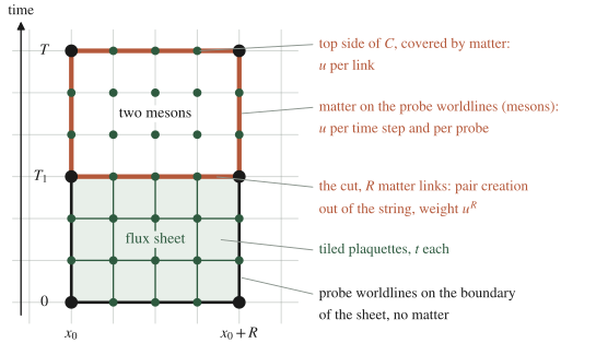
Figure 2. The flux tube’s tiled surface cut by a matter-line pair: below $T_1$ the string (weight $t^R$ per row), above it two mesons ($u^2$ per row); the cut and the top side are the pair’s creation and annihilation lines, $u^R$ each.

5.3 A check on the strip

The leading configurations are planar, so the formulas hold in every $d$, and we checked them against the two-dimensional model, where they can be computed exactly on an open strip of 11 sites: $V(R)=\ln ({\lambda }_0/{\lambda }_R)$ from the unitary-gauge transfer matrix, with the two temporal Wilson lines inserted in ${\lambda }_R$. At $(\beta ,\kappa )=(0.3,0.1)$ the leading order gives $\sigma =1.23336$, $2E_M=4.61182$ and $R_{\ast }=3.74$, and the exact potential is

$R$	1	2	3	4	5	6	7
$V(R)$, exact	1.23303	2.46606	3.69908	4.59573	4.59573	4.59573	4.59573
$\min (\sigma R,2E_M)$	1.23336	2.46672	3.70007	4.61182	4.61182	4.61182	4.61182

The rise is linear, with slope 1.23303, through $R=3$, and the plateau starts at $R=4$, as $R_{\ast }=3.74$ predicts; the small offsets are the next-order corrections of Problem 2. The mixing of §5.2 is visible at the crossing: tuning κ at fixed β so that the two lowest levels at $R=3$ come closest, the exact gap is $1.20\times 2u^3$ at $\beta =0.08$ and $1.43\times 2u^3$ at $\beta =0.15$, the excess coming from cuts spread over two time slices, which are suppressed by a single power of $t$. In $d=3$ the leading order is unchanged, and the dimension enters the corrections through the $2(d-2)$ cube decorations of the sheet and the $2(d-1)$ directions of the meson’s detours.

Physical picture. A simulation of the static potential with dynamical fundamental matter would see the table above: the confining string of Blocks B–C up to $R_{\ast }$, then a plateau at which the ground state of the static pair is two mesons. The area law is an intermediate-distance phenomenon, and the bound $⟨W⟩\ge (\tanh \kappa {)}^{|C|}$ of §2.4 says that it can never be the asymptotic behaviour. The flattening of the static potential by light quarks in QCD, also called string breaking, is the same mechanism in a harder theory [Heuristic]. What replaces the area law as the signature of confinement is taken up in §7 and in Week 14.

6. The analyticity argument of Osterwalder–Seiler and Fradkin–Shenker [Model proof.]

The activity bounds and the counting are proved here for the ${\mathbb{Z}}_2$ model; the convergence criterion for polymer gases is quoted [Stated — refs: Kotecký & Preiss, Commun. Math. Phys. 103 (1986) 491]; the case of continuous gauge groups is Osterwalder and Seiler’s [Stated — refs].

6.1 Polymer gases and a convergence criterion

A polymer gas is a set of polymers γ with complex activities $w(\gamma )$ and a symmetric incompatibility relation, each polymer being incompatible with itself; its partition function is $\Xi =\sum \prod w(\gamma )$ over families of pairwise compatible polymers. The Kotecký–Preiss criterion states that if, for every polymer ${\gamma }^{\prime }$,

$$\sum _{\gamma \text{incompatible with}{\gamma }^{\prime }}|w(\gamma )|e^{|\gamma |}\le |{\gamma }^{\prime }|,$$

then $\ln \Xi$ is an absolutely convergent sum of cluster terms, each a polynomial in finitely many activities, and the terms that touch a given polymer are bounded by its size. The free energy per site then converges, uniformly in the volume, to an analytic function of the activities, and so do ratios such as $⟨W(C)⟩$ and the truncated correlations of local observables, which decay exponentially.

One counting lemma reduces the criterion to a single inequality. In a graph of maximal degree $D$ the connected sets of $n$ vertices that contain a given vertex number at most $D^{2(n-1)}$, since a depth-first walk around a spanning tree of the set is a closed walk of $2(n-1)$ steps from that vertex and determines the set. If polymers are connected vertex sets with $|w(\gamma )|\le {\epsilon }^{|\gamma |}$, and every polymer incompatible with ${\gamma }^{\prime }$ contains one of at most $(D+1)|{\gamma }^{\prime }|$ vertices, the left side of the criterion is at most $(D+1)|{\gamma }^{\prime }|{\sum }_{n\ge 1}{D}^{2(n-1)}(e\epsilon {)}^n=(D+1)|{\gamma }^{\prime }|e\epsilon /(1-D^{2}e\epsilon )$, and the criterion holds for

$$\epsilon \le {\epsilon }_0=\frac{1}{e(D^2+D+1)}.$$

6.2 Small β, uniformly in κ

By §4.1, $Z\propto {\sum }_S{t}^{|S|}{u}^{|\partial S|}$. Decompose $S$ into its link-connected components, two plaquettes being adjacent when they share a link. Components that share no link have boundaries on disjoint sets of links, so $|S|$ and $|\partial S|$ are additive. The polymers are therefore the link-connected plaquette sets, incompatible when they share a link, with activity $w(\gamma )=t^{|\gamma |}{u}^{|\partial \gamma |}$, and for $|u|\le 1$

$$|w(\gamma )|\le |t{|}^{|\gamma |}\text{uniformly in }\kappa ,$$

a bound that also holds for complex κ with $|\mathrm{Im}\kappa |\le \pi /4$, where $|\tanh \kappa |\le 1$. In $d=3$ a plaquette shares a link with $D=4(2d-3)=12$ others, so ${\epsilon }_0=1/(157e)=2.34\times 10^{-3}$: for $\tanh \beta <2.34\times 10^{-3}$ and every $\kappa \in [0,\infty ]$ the free energy and all local gauge-invariant correlators are analytic and cluster exponentially. The uniformity is the whole point, and its origin is simple: the matter factor $u^{|\partial \gamma |}$ can only make a sheet cheaper.

6.3 Large κ, uniformly in β

Expand around $\sigma \equiv 1$. Let $L$ be the set of reversed links, so that $e^{\kappa \sum {\sigma }_{\ell }}=e^{\kappa N_{\ell }}{v}^{|L|}$ and $e^{\beta \sum {\sigma }_P}=e^{\beta N_P}{y}^{F(L)}$, where $F(L)$ counts the frustrated plaquettes, those that contain an odd number of links of $L$:

$$Z=2^{N_s}{e}^{\kappa N_{\ell }+\beta N_P}\sum _L{v}^{|L|}{y}^{F(L)}.$$

Decompose $L$ into plaquette-connected components, two links being adjacent when they lie on a common plaquette. The links of $L$ on the boundary of any plaquette are mutually adjacent, so each plaquette’s frustration is decided within a single component and $F$ is additive. The polymers are the plaquette-connected link sets, incompatible when adjacent or overlapping, with activity $w(\gamma )=v^{|\gamma |}{y}^{F(\gamma )}$, and for $\mathrm{Re}\beta \ge 0$

$$|w(\gamma )|\le |v{|}^{|\gamma |}\text{uniformly in }\beta \in [0,\infty ].$$

A link is adjacent to $D=6(d-1)=12$ links in $d=3$, the same number as in §6.2, so the expansion converges for $e^{-2\kappa }<2.34\times 10^{-3}$, that is $\kappa >{\kappa }_0=3.03$, at every β, $\beta =\infty$ included, where it is the low-temperature expansion of the Ising model of §3. The coincidence of the two constants is the self-duality: under $(t,u)\to (\tilde{v},\tilde{y})$, which is $\tanh \beta =e^{-2\tilde{\kappa }}$ and $\tanh \kappa =e^{-2\tilde{\beta }}$, the polymers of §6.2 become those of §6.3 on the dual lattice.

6.4 The domain and what follows

The strips $D_1=\{\tanh \beta <t_0\}$ and $D_2=\{\kappa >{\kappa }_0\}$, with the crude values $t_0=2.34\times 10^{-3}$ and ${\kappa }_0=3.03$, overlap in the corner of small β and large κ, so $\mathcal{D}=D_1\cup D_2$ is open and connected (Figure 1). It contains the confinement corner, where β and κ are both small, and the Higgs corner, where both are large. It does not contain the corner of large β and small κ, and no argument of this kind could reach it: there $t\approx 1$ and $v\approx 1$, and the corner is the free-charge phase of §3, separated from the rest by the transitions of §7. Three consequences follow.

1. Complementarity. A path from the Higgs corner to the confinement corner inside $\mathcal{D}$, along the top of the diagram and down its left side, crosses no singularity of the free energy or of any local gauge-invariant correlator.
2. No local order parameter. The expectation value of any local gauge-invariant observable is real-analytic on the connected domain $\mathcal{D}$. If it vanished on an open part of the confinement corner, it would vanish on all of $\mathcal{D}$ by the identity theorem, the Higgs corner included; no local observable can vanish in one regime and not in the other.
3. Lines end. No line of singularities enters $\mathcal{D}$, so none reaches the edges $\beta =0$ and $\kappa =\infty$. On the other two edges the free energy is singular only at $({\beta }_c,0)$ and $(\infty ,{\kappa }_c)$, the transitions of §3, so a line of singularities that starts at neither point, and does not run into the corner of large β and small κ, has no edge to end on and must end in the interior.

For continuous gauge groups the large-κ expansion is no longer a gas of discrete polymers, since the links fluctuate continuously about 1; the needed estimates belong to Osterwalder and Seiler’s treatment of the Higgs mechanism, on which Fradkin and Shenker’s argument rests [Stated — refs: Osterwalder–Seiler 1978; Fradkin–Shenker 1979].

Physical picture. The two strips work by opposite mechanisms. On the left, flux sheets are small and rare whatever the matter does, and the matter only makes them cheaper by letting them end. On the top, reversed links are rare whatever the plaquettes do, and the plaquette term only makes them rarer. In the corner where both hold, the confinement description (dilute sheets, charges bound into mesons) and the Higgs description (links frozen, a massive gauge field) are two convergent expansions of the same functions, and they must agree, which §8 checks on a mass. For the research line of the course the statement reads: condensing the fundamental electric charge (Higgs) and condensing the magnetic defects of Week 5, the visons (confinement), lead to the same phase, and the self-duality of §4.2 makes the statement symmetric, since it exchanges the two condensates (julia-toulouse-mechanism, condensation-defects; forward reference to Semester II, heuristic at this stage).

7. The phase diagram in $d=3$

7.1 Two continuous lines and the multicritical point

The pure-gauge transition persists for small $\kappa >0$ (Fradkin and Shenker present an argument due to Wegner for its stability [Stated — refs: Fradkin–Shenker 1979]), and by the duality of §4.2 so does the Ising transition at large finite β. The two lines bound the free-charge phase at large β and small κ, where static charges are free and the gauge field is in the deconfined, ${\mathbb{Z}}_2$ topologically ordered state of Week 5, the toric-code phase of Semester II Week 8. They are mirror images under the duality, so if they meet at a single point M, it lies on the self-dual line; since $(t_c,u_c)=(0.6419,0.2181)$ satisfies $t+u+tu=1$, M sits near the corner that two straight lines would form. Monte Carlo on lattices up to $60^3$ finds that the two lines stay continuous up to M and merge there into a first-order line [Stated — refs: Tupitsyn et al. 2010]. Condensing either the charge or the vison while the other stays gapped gives 3d Ising exponents, and the self-dual transition out of the deconfined phase at M appears continuous, with large scaling dimensions for all local operators and no known continuum Lagrangian [Stated — refs: Somoza, Serna, Nahum 2021].

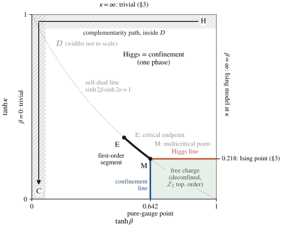
Figure 1. The ${\mathbb{Z}}_2$ gauge–Higgs model in $d=3$: the confinement and Higgs lines bound the free-charge phase and meet at M on the self-dual line, from which a first-order segment runs to the endpoint E; the analyticity domain $\mathcal{D}$ (hatched) contains the trivial edges, and the complementarity path runs inside it from H to C. The shapes of the two lines and the positions of M and E are schematic.

7.2 The first-order segment and its endpoint

From M the first-order line runs along the self-dual line into the Higgs–confinement region [Stated — refs: Tupitsyn et al. 2010]. Two states coexist on it, and the duality exchanges them: approaching a point of the segment from one side, its image approaches from the other. Differentiating the boxed identity of §4.2 with respect to β, with $d{\beta }^{\ast }/d\beta =-1/\sinh 2\beta$, $N_P=N_{\ell }=3N_s$, ${\partial }_{\beta }\ln Z=N_P⟨{\sigma }_P⟩$ and ${\partial }_{\kappa }\ln Z=N_{\ell }⟨s\sigma s⟩$, where $⟨s\sigma s⟩\equiv ⟨s_x{\sigma }_{\ell }{s}_{x+\hat{\mu }}⟩$, gives

$$⟨{\sigma }_P{⟩}_{\beta ,\kappa }=\coth 2\beta -\frac{⟨s\sigma s{⟩}_{{\kappa }^{\ast },{\beta }^{\ast }}}{\sinh 2\beta }.$$

On the self-dual line the dual point is the point itself, with the two coexisting states A (confinement-like) and B (Higgs-like) exchanged, so $⟨{\sigma }_P{⟩}_A=\coth 2\beta -⟨s\sigma s{⟩}_B/\sinh 2\beta$ and the same with A and B exchanged. Subtracting gives, for the jumps $\Delta =B-A$,

$$\sinh 2\beta \Delta ⟨{\sigma }_P⟩=\Delta ⟨s\sigma s⟩\ge 0,$$

both energy densities jumping upward on the Higgs-like side, as the Griffiths monotonicity of §2.4 requires. By consequence 3 of §6.4 the segment cannot reach $\mathcal{D}$, so it ends at a point E in the interior. Beyond E the Higgs-like and confinement-like regions are joined, and a path that passes between E and the edges meets no singularity (Figure 1).

7.3 The liquid–gas analogy [Formal analogy.]

In a simple fluid the liquid and the gas have the same symmetry, the boiling line ends at the critical point, and a path above the critical point takes the liquid to the gas without boiling. “Liquid” and “gas” name the two sides of a first-order line; away from the line there is a single fluid phase. The ${\mathbb{Z}}_2$ gauge–Higgs diagram has the same topology (Figures 1 and 3), element by element:

simple fluid, $(T,p)$	${\mathbb{Z}}_2$ gauge–Higgs, $(\beta ,\kappa )$, $d=3$
solid, distinguished by broken translations	free-charge phase, distinguished by topological order (Week 14; Semester II)
melting and sublimation curves	confinement line and Higgs line
triple point	multicritical point M
boiling line	first-order segment M–E on the self-dual line
critical point	endpoint E
liquid and gas	Higgs-like and confinement-like sides of M–E
density jump	jumps of $⟨{\sigma }_P⟩$ and $⟨s\sigma s⟩$
no symmetry distinguishes liquid from gas	no local order parameter (§6.4) and no 1-form symmetry (§2.4)

Two differences keep this a formal analogy. At a triple point three first-order lines meet, whereas the two lines at M are continuous and M is itself a continuous transition. And the solid is set apart by the breaking of a symmetry, while the free-charge phase is set apart by topological order, which Week 14 and Semester II turn into a statement about emergent 1-form symmetries. With these caveats the lesson is exact: “Higgs” and “confinement” are names for the two ends of one phase, as “liquid” and “gas” are, and the first-order segment separates them only locally.

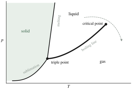
Figure 3. The phase diagram of a simple fluid (schematic), for comparison with Figure 1: the boiling line ends at a critical point, around which liquid and gas are one phase, while the solid is bounded by lines that cannot end.

8. Continuity of the gauge-invariant spectrum

The masses that one calls a massive gauge boson in the Higgs regime and a meson in the confinement regime are read off from one gauge-invariant correlator. Consider the link operator $O_{\ell }=s_x{\sigma }_{\ell }{s}_{x+\hat{\mu }}$ on a spatial link, its connected correlator between times 0 and $n$ along the Euclidean time direction,

$$C(n)=⟨O_{\ell }(0)O_{\ell }(n)⟩-⟨O_{\ell }{⟩}^2,m=-\underset{n\to \infty }{\lim }\frac{1}{n}\ln C(n),$$

and the mass $m$ of the lightest state in this channel. In $\mathcal{D}$ the cluster expansion makes each $C(n)$ analytic and bounds its decay exponentially. Analyticity of each $C(n)$ does not by itself make the decay rate continuous, since an overlap can vanish; that the lightest mass in this channel is isolated and varies continuously along any path in $\mathcal{D}$ is a statement about the transfer matrix, which its own cluster expansion supports and which we assume [Heuristic]. We compute it at the two ends.

8.1 Small β: the meson [Controlled to leading order in $t/(1-u^2)$.]

At $\beta =0$ the links are independent with $⟨{\sigma }_{\ell }⟩=u$. In the expansion of $\ln ⟨{\prod }_P(1+t_P{\sigma }_P)e^{\lambda O_{\ell }(0)+{\lambda }^{\prime }{O}_{\ell }(n)}{⟩}_0$ in independent variables $t_P$, the coefficient of $\lambda {\lambda }^{\prime }$ times a product of distinct $t_P$‘s is the joint cumulant of the corresponding variables. The lowest term connecting $\ell (0)$ to $\ell (n)$ uses the $n$ temporal plaquettes stacked between them, $t^n$ times the joint cumulant of ${\sigma }_{\ell (0)},{\sigma }_{P_1},\dots ,{\sigma }_{P_n},{\sigma }_{\ell (n)}$: a chain in which consecutive members share one link and the others share none. For such a chain each shared link contributes $⟨{\sigma }^2⟩-⟨\sigma {⟩}^2=1-u^2$ and each unshared link $u$; for three members $X=a{\sigma }_1$, $Y={\sigma }_{1}c{\sigma }_2$, $Z={\sigma }_{2}b$,

$$⟨XYZ⟩-⟨XY⟩⟨Z⟩-⟨YZ⟩⟨X⟩-⟨XZ⟩⟨Y⟩+2⟨X⟩⟨Y⟩⟨Z⟩=⟨a⟩⟨b⟩⟨c⟩(1-u^2{)}^2,$$

and induction along the chain gives the rule. The shared links are $\ell (0),\dots ,\ell (n)$, and the unshared ones are the $2n$ temporal links along the two sides of the ribbon, so

$$C(n)=(1-u^2)[t{u}^2(1-u^2){]}^n[1+O(t/(1-u^2))],\boxed{m=\ln \coth \beta +\ln \frac{{\cosh }^4\kappa }{{\sinh }^2\kappa }}$$

at this order. At small κ, $m\simeq \sigma +2E_q$ with $E_q=\ln (1/\kappa )$: two dynamical charges joined by one link of flux, a meson. At large κ, $m\simeq 2\kappa -\ln 4+\ln \coth \beta$: the cost $2\kappa$ of reversing one link in unitary gauge, the massive gauge boson, which needs the plaquette term to move in time. The function is smooth in κ, with its minimum at $\sinh \kappa =1$.

8.2 Large κ: the massive gauge boson [Controlled to leading order in $v/(1-y^2)$.]

In the polymer gas of §6.3, ${\sigma }_{\ell }=-1$ exactly when $\ell \in L$, so $C(n)=4[P(\ell (0),\ell (n)\in L)-P(\ell (0)\in L)P(\ell (n)\in L)]$. At order $v^{n+1}$ the connected part comes from clusters that cover the stack of the $n+1$ copies $\ell (0),\dots ,\ell (n)$ of the link, consecutive copies being adjacent through the temporal plaquette between them. A piece of $m$ consecutive copies frustrates its $2(d-2)m$ spatial plaquettes and the two temporal plaquettes at its ends, the inner temporal plaquettes being reversed twice. The clusters are the ordered decompositions of the stack into $k$ consecutive pieces, whose incompatibility graph is a path, with Ursell coefficient $(-1{)}^{k-1}$:

$$C(n)\simeq 4v^{n+1}{y}^{2(d-2)(n+1)}\sum _{k=1}^{n+1}\left(\genfrac{}{}{0ex}{}{n}{k-1}\right)(-1{)}^{k-1}{y}^{2k}=4v^{n+1}{y}^{2(d-2)(n+1)+2}(1-y^2{)}^n,$$

so that

$$\boxed{m=2\kappa +4(d-2)\beta -\ln (1-e^{-4\beta })}$$

at this order. The factor $(1-y^2{)}^n$ is the plaquette coupling between consecutive copies; at $\beta =0$ it vanishes and the links decouple, as they must. A second family of clusters, the reversal of all links around a column of sites (a gauge transformation of unitary gauge in disguise), costs no frustration and gives the mass $4(d-1)\kappa$, independent of β: it is the Ising particle of the $\beta =\infty$ edge, lighter than the gauge boson only when $4(d-2)\beta -\ln (1-e^{-4\beta })>2(2d-3)\kappa$, close to that edge.

8.3 The corner, and a check

When β is small and κ large, both formulas reduce to

$$m\simeq 2\kappa -\ln (4\beta ),$$

from $\ln \coth \beta \to \ln (1/\beta )$ and $\ln ({\cosh }^4\kappa /{\sinh }^2\kappa )\to 2\kappa -\ln 4$ on the one side, and from $4(d-2)\beta \to 0$ and $-\ln (1-e^{-4\beta })\to -\ln (4\beta )$ on the other. The meson of the confinement description and the gauge boson of the Higgs description are one state seen from two convergent expansions. Each formula is accurate in its own strip, $t\ll 1-u^2$ and $v\ll 1-y^2$ respectively, that is $\beta e^{2\kappa }\ll 1$ and $\beta e^{2\kappa }\gg 1$, and in the corner the crossover between them is governed by $\beta e^{2\kappa }$ (Problem 8⋆⋆). The table gives the exact mass of the two-dimensional model on the strip of §5.3, from the connected correlator at $n=7,8$ of $O_{\ell }$ on the central link of the strip, along a path from the confinement corner to the Higgs corner inside $\mathcal{D}$, together with the two formulas in their $d=2$ form:

$(\beta ,\kappa )$	(0.05, 0.2)	(0.05, 0.6)	(0.05, 1.2)	(0.05, 2.0)	(0.2, 2.5)	(0.6, 2.5)	(1.2, 2.5)
exact	6.2778	4.5657	4.5742	5.7987	5.6149	5.0983	5.0080
§8.1 (small β)	6.2816	4.5802	4.5478	5.7198	5.2767	4.2758	3.8360
§8.2 (large κ)	2.1078	2.9078	4.1078	5.7078	5.5966	5.0951	5.0083

The exact mass changes smoothly along the whole path, the small-β formula tracks it on the left side and the large-κ formula on the top, and at $(0.05,2.0)$, in the corner, both are within 2%.

9. The Hamiltonian face: the toric code in two fields [Computed.]

In $2+1$ dimensions put Pauli operators ${\tau }_v^{x,z}$ on the sites, with ${\tau }_v^x=-1$ meaning a charge at $v$. The ${\mathbb{Z}}_2$ Kogut–Susskind Hamiltonian of Week 7 §7.1 with matter is

$$H=-\Gamma \sum _{\ell }{\sigma }_{\ell }^x-K\sum _P{B}_P-h\sum _v{\tau }_v^x-J\sum _{\ell =⟨vw⟩}{\tau }_v^z{\sigma }_{\ell }^z{\tau }_w^z,{\tau }_v^x\prod _{\ell \ni v}{\sigma }_{\ell }^x=1,$$

where the Gauss law is that of conventions §4, ${\prod }_{\ell \ni v}{\sigma }_{\ell }^x=(-1{)}^{q_v}$, with the dynamical charge $(-1{)}^{q_v}={\tau }_v^x$, $2h$ is the energy of a charge and $J$ its hopping. On the physical subspace define $X_{\ell }={\sigma }_{\ell }^x$ and $Z_{\ell }={\tau }_v^z{\sigma }_{\ell }^z{\tau }_w^z$. Both commute with the Gauss operators, they obey the Pauli algebra link by link, and they act on a space of dimension $2^{N_{\ell }+N_s}/2^{N_s}=2^{N_{\ell }}$, since the $N_s$ Gauss constraints are independent (their product is the total matter parity). The Gauss law gives ${\tau }_v^x={\prod }_{\ell \ni v}{X}_{\ell }\equiv A_v$, and $B_P={\prod }_{\ell \in \partial P}{Z}_{\ell }$ because the ${\tau }^z$ cancel in pairs around a plaquette. Therefore

$$\boxed{H=-h\sum _v{A}_v-K\sum _P{B}_P-\Gamma \sum _{\ell }{X}_{\ell }-J\sum _{\ell }{Z}_{\ell },}$$

the toric code of conventions §9 in a transverse field Γ and a longitudinal field $J$, with the matter charge as the $e$ particle and the vison as the $m$ particle: unitary gauge in Hamiltonian form, and the model of the title of Tupitsyn et al. Its edges repeat §3. At $J=0$ the charges are static, the ground state lies in the charge-free sector, and the model is Week 7’s pure gauge theory, with its transition at $(K/\Gamma {)}_c\approx 3.044$ [Stated — refs: Blöte & Deng, Phys. Rev. E 66 (2002) 066110]. At $\Gamma =0$ the $B_P$ are conserved, the flux-free sector is pure gauge, $Z_{\ell }={\mu }_v^z{\mu }_w^z$ and $A_v={\mu }_v^x$, and $H$ is the transverse-field Ising model $-h\sum {\mu }^x-J\sum {\mu }^z{\mu }^z$ of the matter, with its transition at $(h/J{)}_c\approx 3.044$. The e–m duality of Problem 5⋆ exchanges $(h,\Gamma )$ with $(K,J)$, and the toric-code point $\Gamma =J=0$ lies deep in the free-charge phase: the free-charge phase is the ${\mathbb{Z}}_2$ topological order of the toric code, and the Higgs–confinement phase is its trivial neighbour.

10. Subtleties and fine print

F1 — Fixed versus variable length. Our matter has fixed length, $s=\pm 1$, the limit λ → ∞ of a real scalar φ with potential ${\varphi }^2+\lambda ({\varphi }^2-1{)}^2$; Fradkin and Shenker also work with fixed-length fields. At finite λ both steps of §6 fail as stated. At $\beta =0$ the sum over σ leaves ${\prod }_{\ell }2\cosh (\kappa {\varphi }_x{\varphi }_y)$, an interacting model of the gauge-invariant variable ${\varphi }^2$ with no symmetry at all, which may have a first-order transition of liquid–gas type; and at $\kappa \to \infty$ the links freeze only where $|\varphi |$ is bounded away from zero. The theorem then says nothing, and first-order transitions between Higgs-like and confinement-like regions can occur. The known example is the three-dimensional SU(2)–Higgs model of the hot electroweak theory, whose first-order line ends at a critical point, at $m_H=72(2)$ GeV for ${\sin }^2{\theta }_W=0$, in the 3d Ising class [Stated — refs: Kajantie, Laine, Rummukainen, Shaposhnikov, Phys. Rev. Lett. 77 (1996) 2887; Rummukainen et al., Nucl. Phys. B 532 (1998) 283]: the regions stay connected, as in §7.3, although no convergent expansion proves it.

F2 — The representation of the matter. The trivial edge κ = ∞ is what makes the large-κ strip exist, and it is trivial because the matter is charged under the whole gauge group, so that unitary gauge freezes every link. For $U(1)$ with a Higgs field of charge $q>1$, unitary gauge leaves $a_{\ell }\in \frac{2\pi }{q}{\mathbb{Z}}_q$ at κ = ∞, a ${\mathbb{Z}}_q$ gauge theory with its own confinement transition; the edge is no longer trivial, the argument of §6.3 fails, and a phase boundary may separate the Higgs phase from confinement, as Fradkin and Shenker found for charge $N>1$ and for adjoint $SU(N)$ Higgs fields [Stated — refs: Fradkin–Shenker 1979]. The invariant statement is the residual ${\mathbb{Z}}_{\gcd (N,q)}$ 1-form symmetry of Week 14 (conventions §6).

F3 — What “the Higgs field condenses” depends on. In unitary gauge $s_x=1$ identically, so its “expectation value” is the gauge condition. In the maximal-tree gauge of Week 5 (F2), with σ = 1 on the tree and the matter spin fixed at the root $r$, the same field becomes $s_x=G({\Gamma }_{rx})$ with ${\Gamma }_{rx}$ the tree path, which decays with the length of that path at every finite β and vanishes in the thermodynamic limit. Two complete gauges assign the “Higgs condensate” the values 1 and 0 at the same coupling, and neither is an order parameter; Elitzur’s bound of §2.3 constrains only the unfixed average.

F4 — The endpoint’s universality class. Off the self-dual line no symmetry acts, so the endpoint E has no symmetry-protected order parameter. On the line the duality acts on local observables as a ${\mathbb{Z}}_2$: with Δ the jumps of §7.2, the combination $\sinh 2\beta ⟨{\sigma }_P⟩+⟨s\sigma s⟩-\cosh 2\beta$ equals $\pm \Delta ⟨s\sigma s⟩$ in the two coexisting states and is odd under the duality. Along M–E this ${\mathbb{Z}}_2$ is spontaneously broken and beyond E it is restored, with the distance from the self-dual line acting as its conjugate field, which makes the 3d Ising class the natural expectation for E [Heuristic]. It is the class found at the endpoint of the electroweak line of F1 [Stated — refs: Rummukainen et al. 1998]; for the ${\mathbb{Z}}_2$ model we know of no direct determination.

F5 — Fredenhagen and Marcu. Something must distinguish the free-charge phase from the rest, since transitions separate them. Fredenhagen and Marcu constructed finite-energy charged states in the ${\mathbb{Z}}_2$ gauge–Higgs model [Commun. Math. Phys. 92 (1983) 81] and later proposed the order parameter

$${\rho }_{\mathrm{FM}}=\underset{R,T\to \infty }{\lim }\frac{G({\Gamma }_{R,T})}{⟨W(C_{R\times T}){⟩}^{1/2}},$$

where ${\Gamma }_{R,T}$ is the half of the rectangle $C_{R\times T}$ below its horizontal midline, with matter at the two ends, a distance $R$ apart [Phys. Rev. Lett. 56 (1986) 223]. The square root cancels the perimeter self-energy of the line, and ${\rho }_{\mathrm{FM}}$ tends to zero where a charge cannot be screened, the free-charge phase, and to a nonzero constant where it is screened [Stated — refs: Fredenhagen–Marcu 1986]. It is gauge invariant and nonlocal, and it measures no symmetry. Problem 3 evaluates it on the edges.

F6 — Other dimensions. The arguments of §§2, 3, 5 and 6 hold in any $d\ge 2$, with $D=4(2d-3)$ and $6(d-1)$ in §6. In $d=4$ the edge κ = 0 has the first-order transition at 0.4407 (Week 5 §8.3) and the edge β = ∞ the 4d Ising transition, and there is no self-duality with matter: plaquettes are dual to plaquettes, and the relabeling of §4.2 produces a ${\mathbb{Z}}_2$ two-form gauge field. In $d=2$ the edge κ = 0 has no transition (Week 5 §6), and the model served here only as an exactly computable test of the leading orders.

F7 — Crude constants and the true region. The values $t_0=2.34\times 10^{-3}$ and ${\kappa }_0=3.03$ are artefacts of the criterion; the Monte Carlo studies of §7 find singularities only on the lines of Figure 1. The theorem guarantees analyticity on $\mathcal{D}$ only, and the first-order segment is a genuine singularity inside the “one phase”: local observables jump across it. “One phase” means connected by paths of analyticity, as for the fluid.

11. Common misconceptions

• “The Higgs mechanism breaks the gauge symmetry, and $⟨\varphi ⟩\ne 0$ is its order parameter.” It is tempting because in a fixed gauge the scalar has a nonzero expectation value and textbook language says the symmetry is broken. A gauge symmetry is a redundancy of the description, and Elitzur’s theorem forbids its breaking (§2.3). In unitary gauge $⟨{\sigma }_{\ell }⟩\ge \tanh \kappa$ at every $\kappa >0$, deep in the confinement regime included (§2.4), and two complete gauges give the “condensate” the values 1 and 0 (F3). The Higgs phenomena, a massive vector boson and screened charges, are properties of gauge-invariant correlators (§8), which is the content of the general analysis of Fröhlich, Morchio and Strocchi [Stated — refs: Nucl. Phys. B 190 (1981) 553].
• “Higgs and confinement are distinguished by the Wilson loop: perimeter law in the Higgs phase, area law in the confining phase.” It is tempting because in the pure gauge theory the area law is the order parameter of confinement and a Higgs phase screens charges. With fundamental matter $⟨W(C)⟩\ge (\tanh \kappa {)}^{|C|}$ at every β (§2.4), so the perimeter law holds everywhere; the area law is the behaviour below $R_{\ast }$ (§5), and the 1-form symmetry that the loop diagnoses is explicitly broken (conventions §6). The loop distinguishes phases only at κ = 0, or with matter that leaves part of the center unbroken (Week 14).
• “The Higgs and confinement regimes are connected because the expansions converge at large β or at large κ.” It is tempting because both large couplings simplify, and the weak-coupling expansion of Week 5 does converge at κ = 0. The domain is small β at every κ together with large κ at every β (§6). At large β and small κ the model is in the free-charge phase, separated from the rest by transitions (§7); the argument works because each of its two strips contains a trivial edge and its activity bound is uniform in the other coupling.

12. Historical note

Fradkin and Shenker’s paper, “Phase diagrams of lattice gauge theories with Higgs fields”, studies lattice gauge theories coupled to fixed-length scalar fields for the groups ${\mathbb{Z}}_2$, $U(1)$ and $SU(N)$. Its central result is that when the Higgs field transforms like the fundamental representation the Higgs and confining regimes are smoothly connected, with no phase boundary between them, while for other representations (all Higgs fields in the adjoint of $SU(N)$, or of charge $N>1$ for $U(1)$) a boundary may exist. The paper also presents an argument due to Wegner for the stability of the pure-gauge transition, and it identifies a third regime, the free-charge or Coulomb phase, whose spectrum contains finite-energy states that represent free charges, together with massless gauge bosons for continuous groups. The analytic connection rests on the rigorous work of Osterwalder and Seiler, whose paper of 1978 proved reflection positivity and the existence of a positive transfer matrix for lattice gauge theories, established the existence and analyticity of the strongly coupled infinite-volume limit with Wilson’s confinement bound, and gave a rigorous treatment of the Higgs mechanism on the lattice. The model proof of §6, with its constants, is the course’s own version for ${\mathbb{Z}}_2$, where discreteness makes both expansions polymer gases; the result is now usually called Higgs–confinement complementarity. The numerical diagram came later: early Monte Carlo work by Jongeward, Stack and Jayaprakash (1980), and three decades afterwards the large-lattice study of Tupitsyn, Kitaev, Prokof’ev and Stamp (2010), which found the multicritical point, followed by the analysis of its self-dual criticality by Somoza, Serna and Nahum (2021).

13. What to take away

1. Charge-1 matter adds the hopping κ, and unitary gauge turns it into a link field (§2.2). Elitzur’s theorem still forbids local order [Proved], and the unitary-gauge link expectation is at least $\tanh \kappa$ in every phase, so it is an energy density and no order parameter.
2. The Wilson loop obeys $⟨W(C)⟩\ge (\tanh \kappa {)}^{|C|}$ at every β [Proved]. The flux tube breaks at $R_{\ast }=2\ln \coth \kappa /\ln \coth \beta$, where a string state and a two-meson state cross with a gap $2u^{R_{\ast }}$ [Controlled]; the electric 1-form symmetry is explicitly broken.
3. Two edges are trivial and two carry one transition each (β_c = 0.7614 at κ = 0, κ_c = 0.2217 at β = ∞). In $d=3$ the exact self-duality $Z(\beta ,\kappa )=(\sinh 2\beta \sinh 2\kappa {)}^{3N_s/2}Z({\kappa }^{\ast },{\beta }^{\ast })$ exchanges them and makes the two transition lines mirror images.
4. The free energy is analytic for small β at every κ and for large κ at every β, because each expansion’s activity bound is uniform in the other coupling [Model proof]. The corner of large β and small κ, the free-charge phase, is excluded. Higgs and confinement are one phase, and the first-order segment inside it must end, at a critical point, as the boiling line of a fluid does.
5. The gauge-invariant spectrum interpolates. One mass in the channel $s\sigma s$ is a meson at small κ and a massive gauge boson at large κ, and the two expansions give the same $2\kappa -\ln 4\beta$ in the corner (§8).

14. Looking ahead: Week 14

If Higgs and confinement are one phase for fundamental matter, when are there distinct phases, and what distinguishes them? Week 14 answers with the center of the gauge group. Matter of charge $q$ in a ${\mathbb{Z}}_N$ gauge theory leaves a residual ${\mathbb{Z}}_{\gcd (N,q)}$ 1-form symmetry, whose realization separates phases without any local order parameter; Polyakov loops and ‘t Hooft’s flux sectors make it concrete, and the charge-2 Higgs phase of Hansson, Oganesyan and Sondhi turns out to be topologically ordered. The free-charge phase of this week, the toric-code phase, is the first example, and the edge κ = ∞ of F2 is where the arithmetic of $\gcd (N,q)$ enters.

15. Problem set

Problems 1–3 are the classroom core and are solvable from the note alone; Problems 4⋆ and 5⋆ are self-study consolidation, each with a hint; Problems 6⋆⋆–8⋆⋆ are research extensions that state what is known, what is explored, the sources they need and what counts as completion.

Core problems (everyone).

1. Energy densities under the duality. (Extends §§4.2 and 7.2.) (a) §7.2 derives the first relation below from the boxed identity of §4.2. Derive the second in the same way:

$$⟨{\sigma }_P{⟩}_{\beta ,\kappa }=\coth 2\beta -\frac{⟨s\sigma s{⟩}_{{\kappa }^{\ast },{\beta }^{\ast }}}{\sinh 2\beta },⟨s\sigma s{⟩}_{\beta ,\kappa }=\coth 2\kappa -\frac{⟨{\sigma }_P{⟩}_{{\kappa }^{\ast },{\beta }^{\ast }}}{\sinh 2\kappa }.$$

(b) Show that $⟨s\sigma s⟩=u+2(d-1)t{u}^3(1-u^2)+O(t^2)$ at small β and $⟨s\sigma s⟩=1-2v{y}^{2(d-1)}+O(v^2)$ at large κ, and check both against the Griffiths bound. (c) Insert the small-β result of (b) at the dual point into (a) to obtain $⟨{\sigma }_P⟩$ at large κ in $d=3$, and confirm it by counting reversed links directly. (d) Apply the second relation of (a) to the two coexisting states of §7.2 and show that it gives $\sinh 2\kappa \Delta ⟨s\sigma s⟩=\Delta ⟨{\sigma }_P⟩$. Show that on the self-dual line this is the jump relation of §7.2, and say which identity between β and κ makes the two agree.

2. String breaking at the next order. (Extends §5.) For a planar $R\times T$ loop with $t,u\ll 1$: (a) Show that one-plaquette holes in the flat sheet, bounded by a matter loop, and the cube decorations of Week 5 change the tension to $\sigma =-\ln t-u^4(t^{-1}-t)-2(d-2)t^4+\dots$. (b) Show that detours of a meson’s matter worldline around strips of $n$ plaquettes lower its rest energy to $E_M=-\ln u-2(d-1)[u^{2}t/(1-t)-t{u}^4/(1-t{u}^2)]+\dots$. (c) Evaluate (a) and (b) at $(\beta ,\kappa )=(0.3,0.1)$ in $d=2$, compare with the strip values of §5.3, and give $R_{\ast }$ at this order. (d) Explain why no correction of this kind can restore an area law at large $R$.

3. The open Wilson line and the Fredenhagen–Marcu ratio. (Extends §§2.4 and 3 and F5.) (a) §3 gives $G(\Gamma )$ on the four edges: at β = 0 it depends only on the length of Γ, at β = ∞ only on its endpoints. At small β, compute the first correction in $t$ for a straight line of length $n$ and for a line of the same length with one right-angle corner (infinite lattice, $d=3$), and show that the ratio of the two is $1+t(1-u^2{)}^2+O(t^2)$: away from the edge $G$ depends on the shape of Γ. (b) Compute ${\rho }_{\mathrm{FM}}$ on the four edges. (c) At small β and small $\kappa >0$, evaluate ${\rho }_{\mathrm{FM}}$ at leading order for loops with $R>R_{\ast }$. Compare with κ = 0, and explain why the limits κ → 0 and $R,T\to \infty$ do not commute.

Starred problems (Ph.D. expected; ambitious M.Sc. encouraged).

4⋆. Test a claim: the 1-form symmetry generator with matter. Claim: “Reversing β on the plaquettes pierced by a closed dual loop $\tilde{\Sigma }$ is still a change of variables when matter is present, so $⟨U(\tilde{\Sigma })⟩=1$ in every phase.” (a) Repeat the substitution $\sigma \to \sigma \lambda$ of Week 5 §8.1 and find what it does to the hopping term. (b) Compute $⟨U(\tilde{\Sigma })⟩$ at leading order in $t$ for a planar dual loop that pierces $|F|$ plaquettes. (c) Decide the claim, and state what it implies for the electric 1-form symmetry (conventions §6). (Hint: in the surface expansion $U$ changes $t\to -t$ on $F$, and the lowest term that notices it is a one-plaquette sheet with a matter loop on its boundary.)

5⋆. The e–m duality of the Hamiltonian. For the Hamiltonian of §9 on the plane: (a) put Pauli operators on the dual links and show that ${\tilde{X}}_{{\ell }^{\ast }}=Z_{\ell }$, ${\tilde{Z}}_{{\ell }^{\ast }}=X_{\ell }$ maps $H(h,K,\Gamma ,J)$ to $H(K,h,J,\Gamma )$ on the dual lattice; (b) show that this is the time-continuum limit of the duality of §4.2 applied to the anisotropic model of Week 7 §2, with $e^{-2{\beta }_t}=a_t\Gamma$ and ${\beta }_s=a_{t}K$ for the gauge field and $e^{-2{\kappa }_t}=a_{t}h$ and ${\kappa }_s=a_{t}J$ for the matter; (c) locate on the self-dual line $h=K$, $\Gamma =J$ the toric-code point and the trivial limits. (Hint: in (b) the dual of a temporal plaquette is a spatial dual link, and the dual of a temporal link is a spatial dual plaquette.)

⋆⋆ problems (research extension; optional).

6⋆⋆. The $U(1)$ diagram with charge-1 and charge-$q$ matter in $d=4$. What is known. Fradkin and Shenker treat $U(1)$ with fixed-length Higgs fields: for charge 1 the Higgs and confinement regimes are connected and a Coulomb phase appears at large β and small κ; for charge $N>1$ a phase boundary may exist. What is explored. The analogue of §§3 and 6 for $S=\beta {\sum }_P(1-\cos (da{)}_P)-\kappa {\sum }_{\ell }\cos ({\phi }_{x+\hat{\mu }}-{\phi }_x-q{a}_{\ell })$. Sources: Fradkin–Shenker 1979; Weeks 6 and 11; Week 14. Completion: the four edges derived, with the transition of Week 11 on κ = 0, the 4d XY model on β = ∞, and the edge κ = ∞ trivial for $q=1$ and a ${\mathbb{Z}}_q$ gauge theory for $q>1$; an account of which steps of §6 survive for a continuous group and which need Osterwalder and Seiler’s estimates; both diagrams sketched, with each line justified or labelled as numerical input.

7⋆⋆. Scaling at the critical endpoint. What is known. The segment M–E on the self-dual line [Tupitsyn et al. 2010]; the duality-odd and duality-even local combinations (F4; Somoza et al. 2021); the 3d Ising class at the electroweak endpoint [Rummukainen et al. 1998]. What is explored. Whether E is in the 3d Ising class, and how its scaling fields sit in the $(\beta ,\kappa )$ plane. Sources: the three papers above, F4 and Problem 1(d). Completion: an argument that the distance from the self-dual line is a field-like scaling variable and the distance along it a thermal-like one, so that the jump of the odd combination vanishes as $|g-g_E{|}^{{\beta }_I}$ along the line; and either a Monte Carlo study in unitary gauge ($L\le 32$) that locates E through the Binder cumulant of the odd combination and compares it with the 3d Ising value, or a critical reading of published data that does the same.

8⋆⋆. Correlator interpolation along the complementarity path. What is known. The two formulas of §8, their agreement at leading order in the corner, and the strip values of §8.3. What is explored. A description of the crossover at $\beta e^{2\kappa }\sim 1$. A candidate follows the link in time as an Ising chain with nearest-neighbour coupling $K$ and field $h$, obtained by averaging the two temporal links of each temporal plaquette and the other links of each spatial plaquette at their value $u$: $\tanh K=\tanh \beta {\tanh }^2\kappa$ and $h=\kappa +2(d-2)\mathrm{artanh}(\tanh \beta {\tanh }^3\kappa )$. Sources: §§6 and 8; Week 4 for the Ising chain. Completion: a proof that the chain’s mass reproduces both formulas of §8 in their limits; a comparison with the strip values of §8.3, which in $d=2$ the chain should match to better than one percent along the whole path (at $(0.05,2.0)$ it gives 5.8046 against the exact 5.7987); and an estimate of its error in $d=3$, from the next order of either expansion or from a transfer matrix on a small cross-section.

Self-study answer checkpoints

These checkpoints cover the core problems; starred and ⋆⋆ problems remain source-led.

1. Energy densities. The decisive step is the chain rule: $\ln Z=\frac{3}{2}{N}_s\ln (\sinh 2\beta \sinh 2\kappa )+\ln Z({\kappa }^{\ast },{\beta }^{\ast })$, with $d{\beta }^{\ast }/d\beta =-1/\sinh 2\beta$, $N_P=N_{\ell }=3N_s$ and ${\partial }_{\beta }\ln Z=N_P⟨{\sigma }_P⟩$, ${\partial }_{\kappa }\ln Z=N_{\ell }⟨s\sigma s⟩$. (b) Each of the $2(d-1)$ plaquettes that contain ℓ contributes $t(⟨{\sigma }_{\ell }{\sigma }_P{⟩}_0-⟨{\sigma }_{\ell }{⟩}_0⟨{\sigma }_P{⟩}_0)=t{u}^3(1-u^2)$; at large κ, ℓ is reversed with probability $v{y}^{2(d-1)}$, all its plaquettes frustrated. Both exceed $\tanh \kappa$ at this order, the second because $1-2v{y}^{2(d-1)}\ge 1-2v\simeq \tanh \kappa$. (c) At the dual point $\tilde{t}\simeq v$ and $\tilde{u}=y$, so $⟨s\sigma s{⟩}_{{\kappa }^{\ast },{\beta }^{\ast }}=y+4v{y}^3(1-y^2)$; with $\coth 2\beta -y/\sinh 2\beta =1$ and $(1-y^2)/\sinh 2\beta =2y$, $$⟨{\sigma }_P⟩=1-8v{y}^4+O(v^2),$$ which is $1-2\times 4v{y}^4$, four links per plaquette. Complete enumeration of the $2^3$ torus reproduces the coefficients of (b) and (c) and the relations (a) to $10^{-19}$. (d) As in §7.2 the image of state A is state B, so $⟨s\sigma s{⟩}_A=\coth 2\kappa -⟨{\sigma }_P{⟩}_B/\sinh 2\kappa$ and the same with A and B exchanged; subtracting gives $\sinh 2\kappa \Delta ⟨s\sigma s⟩=\Delta ⟨{\sigma }_P⟩$. On the self-dual line $\kappa ={\beta }^{\ast }$, and $\sinh 2\beta \sinh 2{\beta }^{\ast }=1$ turns this into $\sinh 2\beta \Delta ⟨{\sigma }_P⟩=\Delta ⟨s\sigma s⟩$, the relation of §7.2; both jumps are nonnegative because both densities are nondecreasing in κ (§2.4). Common failure mode: treating the image of a coexisting state as the same state, which gives the opposite sign and contradicts the monotonicity.
2. String breaking at the next order. In the numerator the hole $S_0\oplus P$ costs $u^4/t$ relative to $S_0$, while the vacuum bubble at $P$, weight $t{u}^4$, which the denominator contains, cannot occur there; per plaquette of $S_0$ the ratio is $(1+u^4/t)/(1+t{u}^4)$. A detour around the strip of $n$ plaquettes next to a probe adds two matter links and $n$ plaquettes, $t^n{u}^2$, minus the vacuum bubble of the same strip, $t^n{u}^{2n+2}$; the sum over $n$ and over the $2(d-1)$ transverse directions gives (b). At $(0.3,0.1)$ in $d=2$: $\sigma =1.23336-0.00031=1.23305$ against the exact slope 1.23303, and $2E_M=4.61182-2(0.00817-0.00006)=4.59560$ against the exact plateau 4.59573, so $R_{\ast }=3.727$. (d) By §2.4, $⟨W⟩\ge u^{2(R+T)}$ at every order. Common failure mode: keeping only the $n=1$ detour, $2t{u}^2$, which at $t=0.29$ misses almost a third of the shift of $E_M$.
3. The open line. (a) Expanding $e^{\beta {\sigma }_P}\propto 1+t{\sigma }_P$ about independent links, $G=u^{|\Gamma |}[1+t{\sum }_P(u^{|\Gamma △\partial P|-|\Gamma |}-u^4\left)\right]+O(t^2)$: a plaquette that shares one link with Γ contributes $u^2-u^4$, one that shares two links contributes $1-u^4$, and the others cancel against the denominator. The straight line has $2(d-1)n$ plaquettes of the first kind; the bent line has $2(d-1)n-2$ of the first kind and one of the second, the plaquette of the corner, so the ratio is $1+t[(1-u^4)-2(u^2-u^4)]=1+t(1-u^2{)}^2$. (Enumeration of a $4\times 4$ open lattice in $d=2$, where the same counting holds, gives the ratio minus one equal to $0.991t(1-u^2{)}^2$ at $\beta =0.01$, $\kappa =0.5$, the difference being of order $t^2$.) (b) ${\rho }_{\mathrm{FM}}=u^{R+T}/(u^{2(R+T)}{)}^{1/2}=1$ at β = 0, and 1 at κ = ∞; at β = ∞, ${\rho }_{\mathrm{FM}}=m_I(\kappa {)}^2$, nonzero for $\kappa >{\kappa }_c$ and zero for $\kappa <{\kappa }_c$; at κ = 0, ${\rho }_{\mathrm{FM}}=0$. (c) The numerator is dominated by the matter line along Γ, $u^{R+T}$, and the denominator by the screened loop, $u^{2(R+T)}$, so ${\rho }_{\mathrm{FM}}\to 1$ for every $\kappa >0$; at κ = 0 the numerator vanishes identically, and since $R_{\ast }\to \infty$ as κ → 0 the screened regime recedes to infinity, so the two orders of limits give 1 and 0. Common failure mode: using the area-law sheet in the denominator for loops longer than $R_{\ast }$.

---

Notes prepared for the generalized-symmetries course, Semester I Block D. Rewritten to the note-quality-template standard on 2026-09-28 (first draft 2026-07-01). Last revised 2026-09-29.